Exploring the Bitcoin blockchain using Java

[This is a short summary of material that I prepared for final year project students]

I assume that you already have a vague idea of what a bitcoin is and you have a simple understanding of the mechanisms behind transactions: payments are made to addresses (that are anonymous, in the sense that they cannot be directly linked to a specific individual), and all transactions are public. Transactions are collected in blocks, and blocks are chained together in the blockchain.

You can think of the blockchain as a big database that is continuously updated and is accessible to everyone. You can download the full blockchain using a software like Bitcoin Core. After installing the software, it will take a couple of weeks for your installation to synchronise. Notice that, at the time of writing, the blockchain has a size of over 130 Gb, take this into consideration…

If you have blockchain data available (not necessarily the whole blockchain, you can also work on subsets of it), it can be analysed using Java. You could do all the work from scratch and read raw data from the files etc. Let’s skip this step and use a library instead. There are several options available in most programming languages. I’m going to use Java and the bitcoinj library. This is a big library that can be used to build applications like wallets, on-line payments, etc. I am going to use just its parsing features for this post.

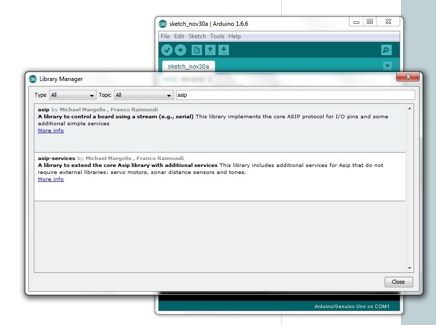
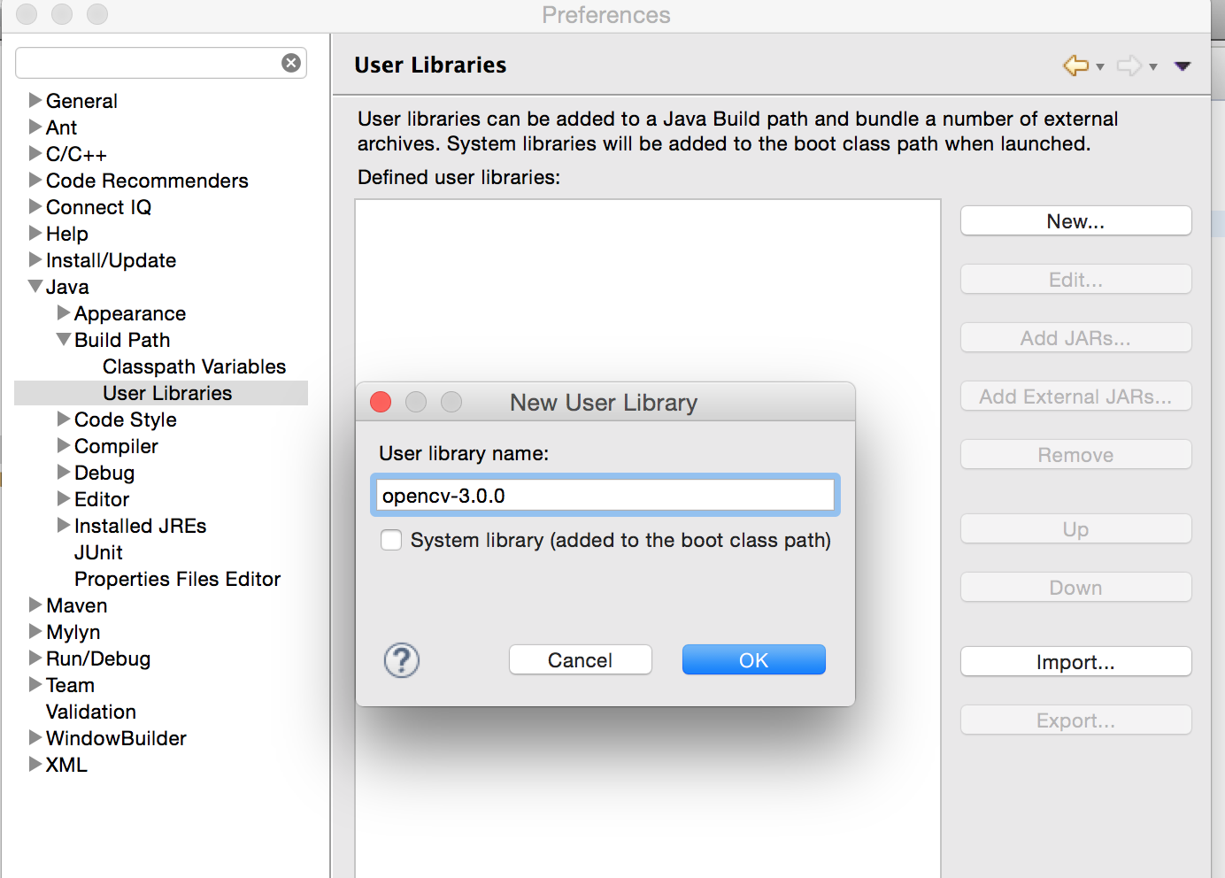
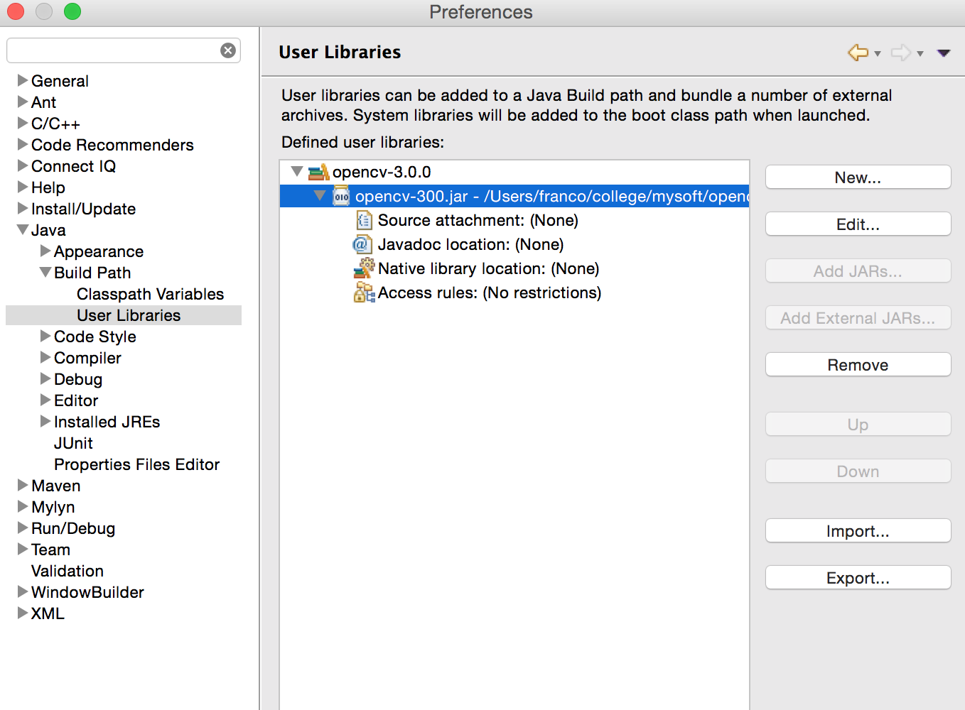
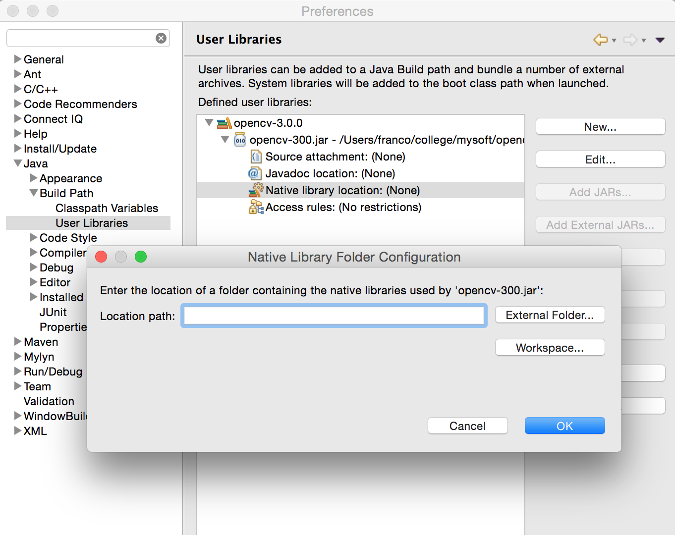
First of all download the jar file for the library at https://bitcoinj.github.io/ (I’m using https://search.maven.org/remotecontent?filepath=org/bitcoinj/bitcoinj-core/0.14.4/bitcoinj-core-0.14.4-bundled.jar). Then, download SLF4J (https://www.slf4j.org/download.html), extract it, and get the file called slf4j-simple-x.y.z.jar (in my case: slf4j-simple-1.7.25.jar). Add these two jar files to your classpath and you are ready to go.

Let’s start from a simple example: compute (and then plot) the number of transactions per day. This is the code, heavily commented, just go through it.

import java.io.File;
import java.text.SimpleDateFormat;
import java.util.LinkedList;
import java.util.List;
import java.util.HashMap;
import java.util.Locale;
import java.util.Map;
 
import org.bitcoinj.core.Block;
import org.bitcoinj.core.Context;
import org.bitcoinj.core.NetworkParameters;
import org.bitcoinj.core.Transaction;
import org.bitcoinj.params.MainNetParams;
import org.bitcoinj.utils.BlockFileLoader;
 
 
public class SimpleDailyTxCount {
 
	// Location of block files. This is where your blocks are located.
	// Check the documentation of Bitcoin Core if you are using
        // it, or use any other directory with blk*dat files. 
	static String PREFIX = "/path/to/your/bitcoin/blocks/";
 
        // A simple method with everything in it
	public void doSomething() {
 
		// Just some initial setup
		NetworkParameters np = new MainNetParams();
		Context.getOrCreate(MainNetParams.get());
 
		// We create a BlockFileLoader object by passing a list of files.
		// The list of files is built with the method buildList(), see
		// below for its definition.
		BlockFileLoader loader = new BlockFileLoader(np,buildList());
 
		// We are going to store the results in a map of the form 
                // day -> n. of transactions
		Map<String, Integer> dailyTotTxs = new HashMap<>();
 
		// A simple counter to have an idea of the progress
		int blockCounter = 0;
 
		// bitcoinj does all the magic: from the list of files in the loader
		// it builds a list of blocks. We iterate over it using the following
		// for loop
		for (Block block : loader) {
 
			blockCounter++;
			// This gives you an idea of the progress
			System.out.println("Analysing block "+blockCounter);
 
			// Extract the day from the block: we are only interested 
                        // in the day, not in the time. Block.getTime() returns 
                        // a Date, which is here converted to a string.
			String day = new SimpleDateFormat("yyyy-MM-dd").format(block.getTime());
 
			// Now we start populating the map day -> number of transactions.
			// Is this the first time we see the date? If yes, create an entry
			if (!dailyTotTxs.containsKey(day)) {
				dailyTotTxs.put(day, 0);
			}
 
			// The following is highly inefficient: we could simply do
			// block.getTransactions().size(), but is shows you
			// how to iterate over transactions in a block
			// So, we simply iterate over all transactions in the
			// block and for each of them we add 1 to the corresponding
			// entry in the map
			for ( Transaction tx: block.getTransactions() ) {		    	
				dailyTotTxs.put(day,dailyTotTxs.get(day)+1);
			}
		} // End of iteration over blocks
 
		// Finally, let's print the results
		for ( String d: dailyTotTxs.keySet()) {
			System.out.println(d+","+dailyTotTxs.get(d));
		}
	}  // end of doSomething() method.
 
 
	// The method returns a list of files in a directory according to a certain
	// pattern (block files have name blkNNNNN.dat)
	private List<File> buildList() {
            List<File> list = new LinkedList<File>();
            for (int i = 0; true; i++) {
                File file = new File(PREFIX + String.format(Locale.US, "blk%05d.dat", i));
                if (!file.exists())
                    break;
                list.add(file);
            }
	    return list;
	}
 
 
	// Main method: simply invoke everything
	public static void main(String[] args) {
		SimpleDailyTxCount tb = new SimpleDailyTxCount();
		tb.doSomething();
	}
 
}

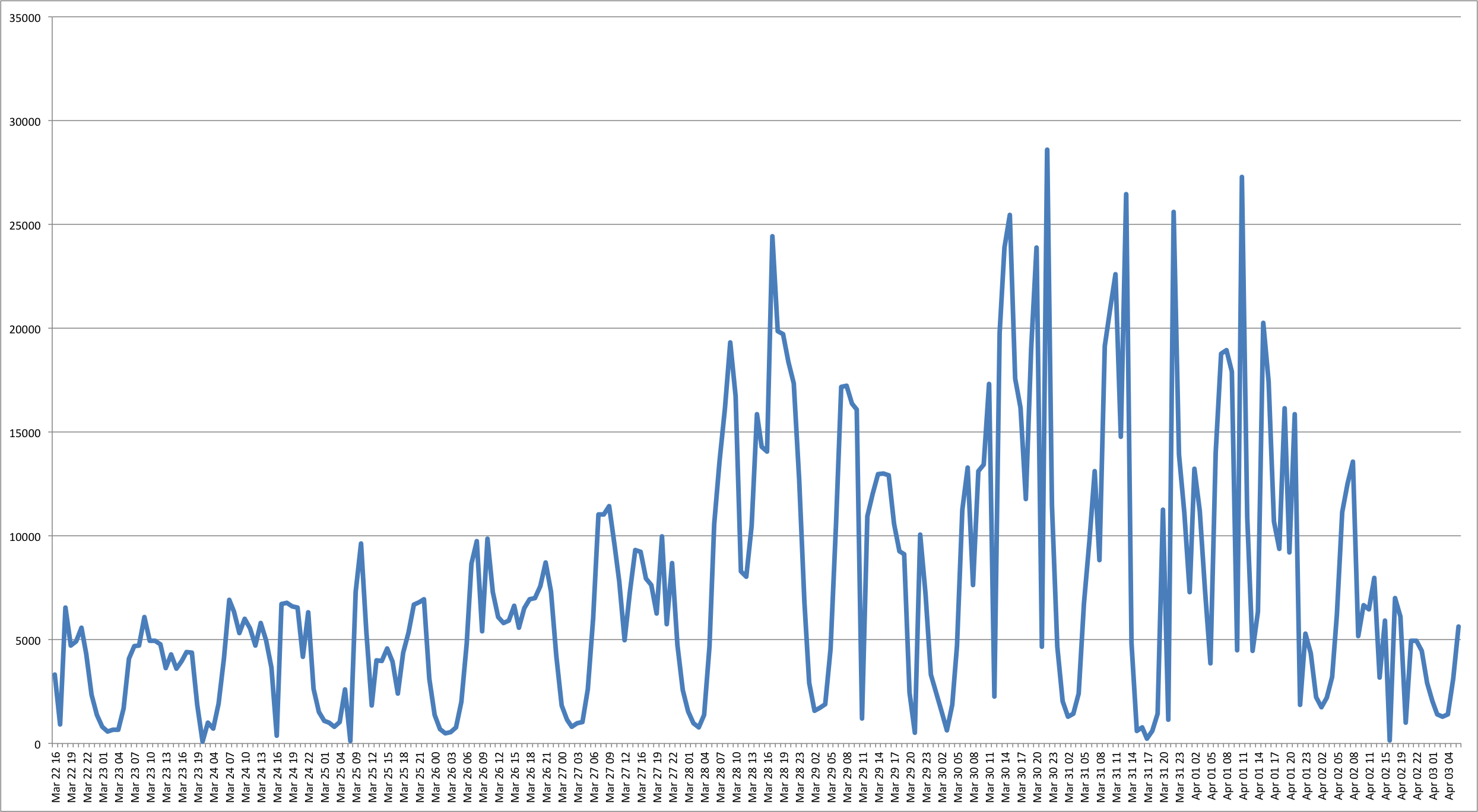
This code will print on screen a list of values of the form “date, number of transactions”. Just redirect the output to a file and plot it. You should get something like this (notice the nearly exponential growth in the number of daily transactions):

dailyTxsLog

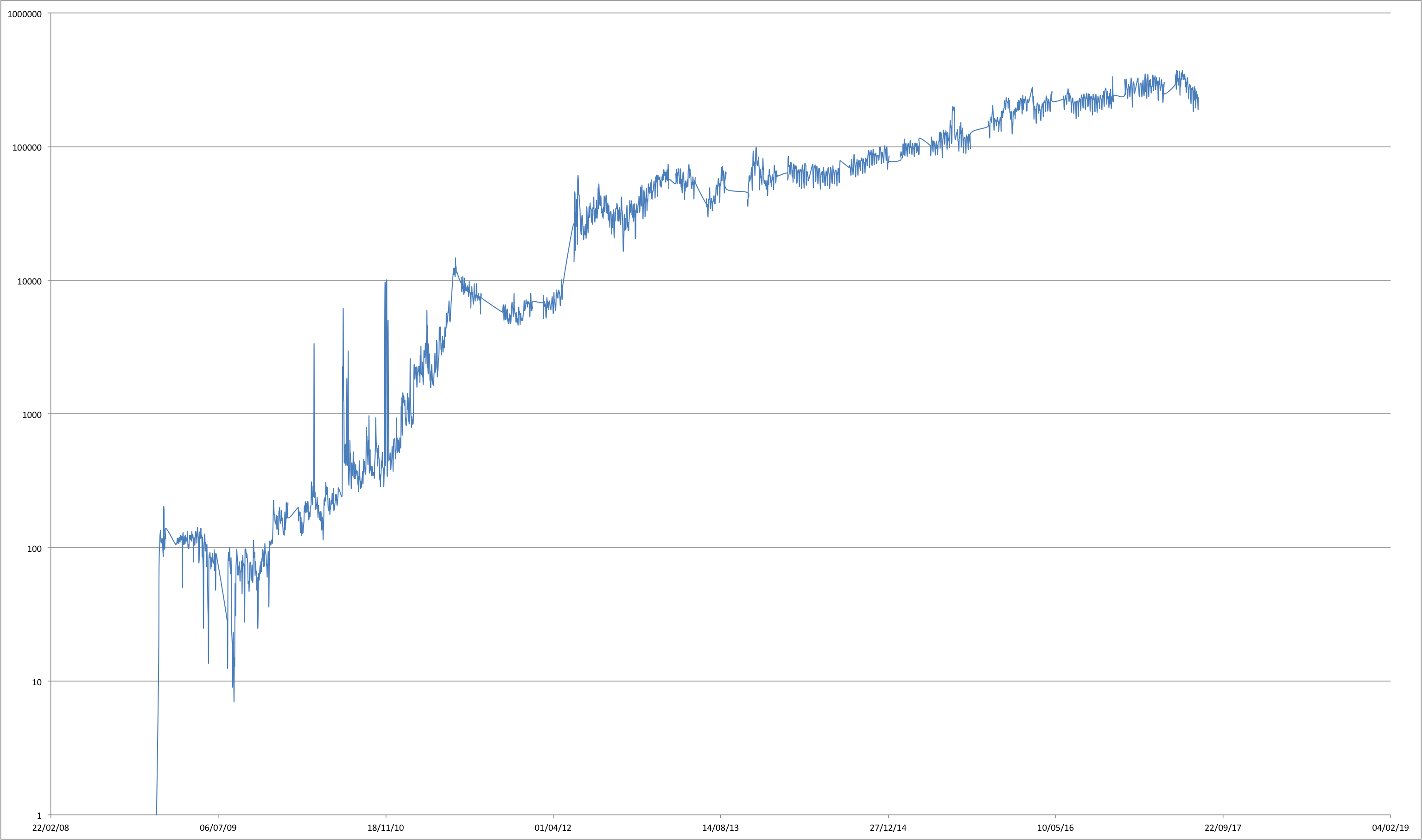
Number of transactions per day (log scale)

I am very impressed by the performance of the library: scanning the whole blockchain with the code above took approximately 35 minutes on my laptop (2014 MacBook Pro), with the blockchain stored on an external HD connected using a USB2 port. It took approximately 100% of one processor and 1 Gb of RAM at most.

A slightly more complicated example took 55 minutes: computing the daily distribution of transaction size. This requires adding a further loop in the code above to explore all the transaction outputs (and a few counters along the way). The buckets are 0-10 USD, 10-50 USD, 50-200 USD, 200-500 USD, 500-2000 USD, 2000+ USD (BTC/USD exchange rate computed by taking the average of opening and close value for the day).

TxSize

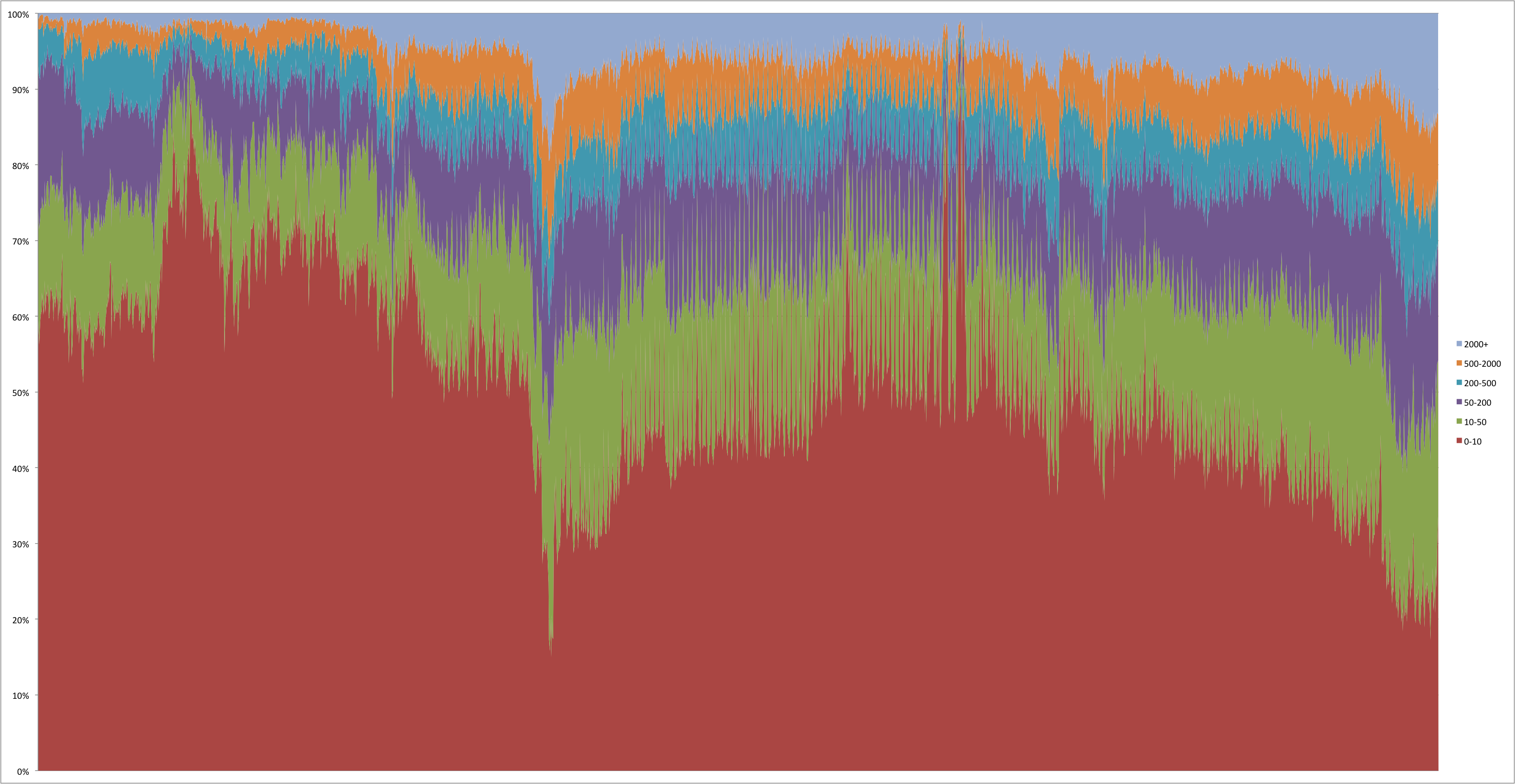
Tx size distribution (in USD), October 2011 – July 2017

On the number of correct answers required in a multiple-choice test

I have been preparing a multiple choice test for our Racket course. The test will consist of 30 questions, each of which has 4 options and only one of them is the correct answer. Students will need to answer to at least 15 questions to pass the test.

Where are these numbers coming from? Why 15 out of 30 and not 12 (40%)? Why 4 options and not 2, with a true/false option only? More importantly: how many questions will be answered correctly by someone selecting random answers?

Let’s suppose that a student is answering randomly. What is the probability that the student answers all questions in the wrong way? This is not difficult to compute: in our case this is (\frac{3}{4})^{30} = 0.0001785. What about one right and 29 wrong? This is \frac{1}{4} multiplied by (\frac{3}{4})^{29}, but you should also remember that there are 30 different ways to get a question right (it could be the first or the second or … or the thirtieth). So, overall, the probability of getting 1 question right and 29 wrong is  30 \cdot \frac{1}{4} \cdot (\frac{3}{4})^{29}. This is nearly ten times more likely than getting all the questions wrong.

In general, what is the probability of getting n questions right and 30-n wrong? This is \frac{1}{4}^n \cdot \frac{3}{4}^{(30-n)}, but we should also multiply this number by the possible combinations of n elements out of 30, that is:

    \[ P(n) = (\frac{1}{4})^n \cdot (\frac{3}{4}))^{(30-n)} \cdot \binom{30}{n} \]

The following is a plot of this function:

prob_correctAs you can see this function has a peak for n=6; the average is \sum n \cdot P(n) = 7.5
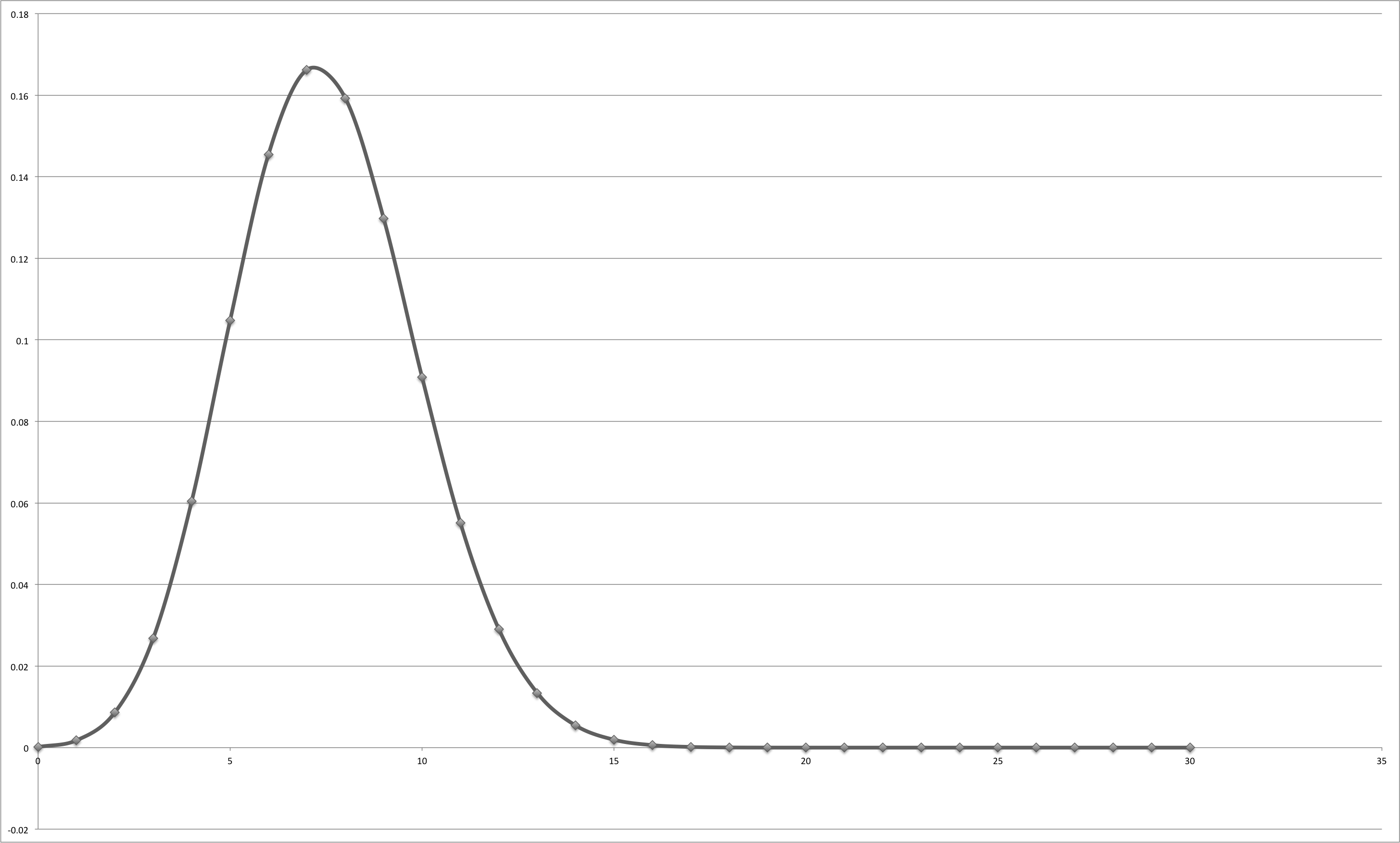
. So, on average, a “random answerer” would get 7.5 questions right. What is the probability of passing the test by answering randomly? We need a cumulative function for this. Let’s plot the probability of passing a test where it is required to answer n questions correctly out of 30 (this is the line in red; the blue line is P(n) as defined above):

cumulative

The probability is obviously 1 if no correct answers are required, and then it decreases reaching 0.001 for n=15
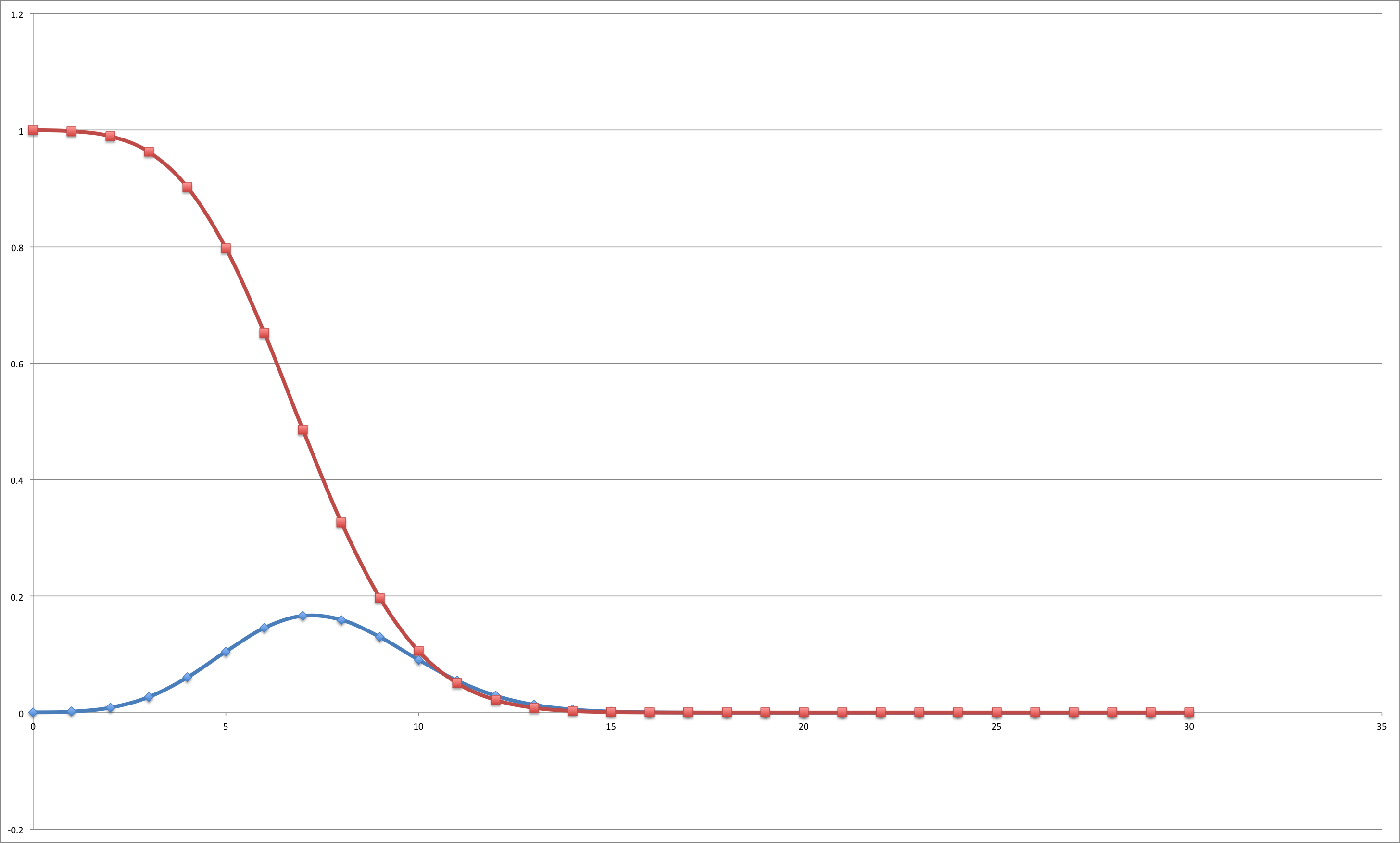
. Going back to the original question: the probability that a student answering randomly passes the test is 0.1%.

[Thanks to Lorenzo Gheri for his input on this :-)]

BBC micro:bit: a very short tutorial

[DISCLAIMER: this is an overly simplified summary, partially taken from a presentation that I gave to a PGCE course. Please refer to https://www.microbit.co.uk/ for proper documentation!]

1071px-bbc_microbit

(source: Wikipedia)

The BBC micro:bit is a microcontroller. You can think of a microcontroller as a simple device that has a set of inputs, a set of outputs, and a piece of code in the middle (called the firmware) that can read the input and write to output. The micro:bit has several input and output options, including: two buttons labelled A and B, 25 LEDs organised in a 5×5 matrix, accelerometer, compass, etc. Writing a program for the micro:bit means creating a firmware to control the output, usually as a reaction to certain input.

You can write programs for the micro:bit using various approaches, some of them are visual (similar to Scratch), some others are textual. This may be a bit confusing at first, but it gives you the opportunity to work with different age groups and to achieve several of the points in the new National Curriculum for Computing, such as “use 2 or more programming languages, at least one of which is textual” in Key Stage 3.

Remember that “writing a program” here means creating a new firmware for the microcontroller. This is done in two steps: first, the code is written and compiled on a standard computer. In fact, you write the code in a browser and you compile it by pressing a button. The result of this operation is a file with .hex extension that you download on your computer. Then, the file needs to be copied on the micro:bit. This last step is very simple: it is enough to connect the micro:bit with its USB cable and copy the file on it.

Suppose that you want to build an application that turns ON the top left LED  when the A button is pressed, and it turns it off when button B is pressed. If you browse to https://www.microbit.co.uk/create-code you will find four different ways to write this program. Let’s start with what I think is the simplest approach: the Microsoft Block Editor. Click on  New Project and you will get an environment that is very similar to Scratch.

The difficult point here is to “design, write and debug [a program] that accomplish[es] specific goals, including controlling or simulating physical systems”, as mentioned in the national curriculum for Key Stage 2. The student should realise that to obtain the behaviour described above some form of loop is needed, together with conditionals (or a mechanism to handle events, which is another option here). The following figure shows a possible solution using a forever loop and two if blocks.

msblockeditorIf you press run you can “test” the program in the browser. If you press compile, you will be able to download a file with .hex extension. Connect the micro:bit to your computer using the USB cable, copy the .hex file that you have downloaded to the micro:bit et voila, the microcontroller is now running the code that you wrote! It will run it forever, until you replace it with another .hex file. You can now disconnect the micro:bit from the computer. Try to power it with the battery pack and press the A button: you will see that the code is running.

You can achieve exactly the same result using MicroPython. Go back to https://www.microbit.co.uk/create-code and click on New Project under Python. You will be presented with a more-or-less plain text editor. You can write Python code, as shown in the following figure:

micropythonThe logic in the figure above is exactly the same: an infinite loop with two if conditions (in this case I have swapped button A and B so that you can verify that the new code is running). Again, as above, pressing the Download button will download a .hex file that you then need to copy to the micro:bit. This approach is less intuitive, as you don’t have a simulator and you can only find out bugs when you upload the code to the device. However, it will only tell you “invalid input” and it’s then up to you to find the problem :-)! You can find additional details about MicroPython here: https://www.microbit.co.uk/python-guide.

If you go back to https://www.microbit.co.uk/create-code you will find two other languages: CodeKingdom JavaScript and Microsoft Touch Develop. The former is essentially JavaScript but, differently from MicroPython, it provides good support with visual blocks that are translated to actual code, in addition to a simulator that can be used to test the code before uploading it to the device. Microsoft Touch Develop is similar in that it provides visual blocks that are then translated into textual code; the syntax of this language is simple enough to be considered nearly pseudo-code and a simulator is available as well.

Hopefully this introduction will allow you to get started. There are many possible extensions: there are built-in functions to create scrolling text on the display and to detect the position of the micro:bit; there is a compass and an accelerometer and a Bluetooth connection is available as well. Additional components can be attached using alligator clips or connected directly with the board, which supports analog input and output (through PWM pins, so that servo motors can be connected as well). You will find plenty of examples on the micro:bit website and online.

If you prefer, you can also program the micro:bit using a tablet or mobile phone: in this case the firmware is transferred using Bluetooth and you need to download an app to enable the transfer (available for Android and iOS).

You could also build applications on a mobile device that access the data on the micro:bit, but this requires programming both the micro:bit and the phone, something that is probably too advanced for this simple tutorial.

What to expect if you are starting Computer Science at Middlesex

We are only one week away from the start of term.  I teach mainly to first year students and for many of them this will be the first experience of higher education. If you are a new student, this is how our teaching is organised: you will spend the vast majority of your time in labs doing something. A lot of people still have a very wrong idea of how learning happens: they imagine that learners are vases to be filled, with teachers standing in front of a class of 20 or so students, “filling” the heads of learners silently seated in front of them. In this vision, the role of the learner is just to remain passive while lectures or lab classes are delivered, and eventually transcribe verbatim what has been taught during an exam a few weeks or months later. In spite of this vision being a few centuries old, it seems to be still shared by many.

This is not what will happen in CS. As a student, most of the time you will be given a handout that you are supposed to read autonomously before coming to your scheduled labs. Some people call it the flipped classroom model, even if what we do is slightly different. We have exceptional new facilities, the rooms where you will work are similar to this one:

room_r209As you can see, the room facilitates working in small groups or individually. Indeed, we know that each student can progress at a different pace and therefore we try to allow students who can go quickly through a topic to progress further, while other students may spend more time on topics that they find hard. In each session there will be academics and teaching assistants and all of us will be happy to switch between different groups working on different topics. We also make heavy use of tools such as Slack and we recommend you to join the team https://mdxcs16.slack.com/ where you will find a number of channels and a lot of people to discuss and ask questions, and we will have a number of drop-in sessions open to support you.

I use often the metaphor of learning to cycle. Learning to code and  learning mathematical concepts is similar to learning how to ride a bicycle. As a teacher, I could tell you on a board with drawings how to do this, and maybe using pictures and videos on slides. You could read a book about cycling and you may even learn racing tactics at Tour de France, writing essays about it and excelling in written exams about the topic. But are you really able to cycle? If you were to join a team at the end of such a cycling course you will be very unlikely to be able to cooperate effectively, and most likely you would struggle simply trying to balance.

Being able of doing Maths and coding are very similar to cycling. As a result, we want to observe you doing it, we don’t want to read your essay about it! Similarly to what happens with a bicycle, you will need to try, try, and try again. This is not going to be a linear process, you need to be persistent and continue trying even if you think that you are not making any progress. What you need is practice, something that you can do in the labs but also with individual study. As teachers, we will not read the handouts to you, you should read the bicycle manual! Our role is to look at how you cycle and suggest improvements; sometimes we may give you a stabilizer if you are leaning on one side, but then we will remove it and we want to observe you cycling alone. This is how you will be assessed: no exams, no essays, but just observation of your behaviours (more on this in another post or, if you are a student, check the handouts!).

The Middlesex Robotic Platform (MIRTO), version 3

MIRTO (also known as Myrtle, or Mirto-bot) is a robotic platform developed at Middlesex University in the School of Science and Technology with the help of staff and students. It has been used in teaching since 2014 and it has been improved in a number of ways during the past two years. The current platform is used not only for teaching, but also for research. In this post I will describe the basic features, some of the applications that have been built on top of it, and the structure of the platform (both software and hardware).

Mirto bot, front view

Mirto, front view

The robot has:

  • Two HUB-ee wheels (with built-in quadrature encoders)
  • Two front bump sensors
  • A small LCD screen (5 lines, 21 characters per line)
  • Infra-red sensors mounted under the base layer (they can be used to follow lines)
  • A potentiometer and a push button
  • A Raspberry Pi layer with WiFi and several other connection points: 4 USB ports, audio output, HDMI output, Ethernet and the usual Raspberry Pi slots for a video camera.

The robot is powered by a standard, rechargeable 5 V battery pack.

Mirto: rear view with battery and Raspberry Pi connections

Mirto: rear view with battery and Raspberry Pi connections

Apart from the hardware characteristics, a substantial amount of effort has been devoted to the development of software to support several programming languages and several mechanisms of interaction with the robot. First year students employ the Racket programming language (a dialect of Lisp) to control the robot. This is an example of Racket code that can be uploaded to the Raspberry Pi and run form there:

(open-asip)
(clearLCD)
(setMotors 180 180)
(setLCDMessage "Starting wheels" 0)
(sleep 1)
(stopMotors)

Alternatively, the robot can be controlled using Java or Python, which can be running either on the Raspberry Pi or on a machine on the same network of the robot, as shown in the following Java example that simulates a simplified Roomba robot:

JMirtoRobotOverTCP robot = new JMirtoRobotOverTCP();
robot.initialize("192.168.42.1"); // Connect to a robot on the same network
robot.setMotors(150,-150);
while (true) {
  if (robot.isPressed(0) || robot.isPressed(1) || (robot.getIR(1)&gt;250)) {
    // Do something if bump sensors pressed or IR reads a value &gt; 250
    robot.stopMotors();
    robot.setMotors(-100,100);
    robot.stopMotors();
    // Now rotate for a bit
    robot.setMotors(100, 100);
    Thread.sleep(500);
    robot.setMotors(150, -150);					
  }
}

Recently, we have developed new blocks for the off-line version of Scratch that can be used to control the robot. The following image shows the new blocks and a Scratch program equivalent to the Java code shown above:

mirto-scratchThe following video shows the results of a program implemented by high school students using Scratch, whose task was to develop a program to keep the robot inside a square marked with black tape (detected by infra-red sensors). The students implemented a program similar to the one in the figure above, adding control of the LCD screen and sounds:

https://www.youtube.com/watch?v=a5AY9LNfXJI

The key software components of Mirto are:

The details of the hardware components of the robot are:

  • A Raspberry Pi. We are currently using a Raspberry Pi 2 Model B (but we are investigating the use of a Raspberry Pi 3).
  • A Teensy 3.2 microcontroller. It has a 32 bit ARM processor, you can think of it as a small but powerful Arduino board with more input and output pins.
  • A bespoke PCB that allows the connection of the Teensy to the Raspberry Pi using the Pi’s GPIO pins and makes it easy to connect all the other components (wheels, bump and infra-red sensors, LCD screen, a piezo buzzer, a potentiometer and a push button)
  • The wheels are two HUB-ee wheels. These wheels have built-in quadrature encoders and can be easily controlled using PWM pins.
  • The perspex layers are cut at Middlesex using a laser cutter. The battery pack is just a standard 9000 mAh battery pack with two USB outputs.

Please feel free to contact me if you need additional details!


Asip now available through Arduino Library Manager

As you probably know if you have read this blog before, Asip is a protocol to control an Arduino board from a computer. The protocol is intended to be a more extensible replacement for Firmata. The idea is that you can control the board directly from a USB or network connection by means of simple plain text messages, such as I,p,13,1 to set pin 13 to high.

From today, installing Asip on an Arduino board is much simpler:

  • Make sure that the version of your Arduino IDE is at least 1.6.2 and open it.
  • Click on Sketch -> Include Libraries -> Manage Libraries to open the library manager.
  • Type asip in the search box and you should get something similar to the following imageArduino library manager for Asip
  • Click on the first link for simple I/O services (you can add support for additional services later with the second link).
  • Click on File -> Examples -> asip and open AsipIO.
  • Connect your board, upload the sketch and you are ready to go.

If you want to use servo motors, sonar distance sensors and piezo tones, in addition to the plain asip library install also the library asip-additional-services and check the examples.

We have developed client libraries in Racket, Java and Python. Contact me if you need additional details, we will try to add tutorials and further documentation as soon as we have time.

Using the Maplin Robotic Arm with Scratch

robotarm-loadtest

Lifting some heavy weights

Maplin is currently selling a robotic arm for £29.99. The arm comes in a box and it needs to be assembled, something that takes approx 2.5 hours. The arm can then be connected to a computer using a USB cable (don’t forget that it also needs 4 D-batteries!). The arm is pretty basic: it has 4 joints and a clamp to hold up to 130 g, but there are no position sensors. This means that you can only move the arm by telling a specific joint to move in a certain direction for a certain amount of time. Nevertheless, I think it is an interesting learning experience and a starting point for other projects (see this video to add position sensors using potentiometers: https://www.youtube.com/watch?v=HDy9jEGMk_k)

In terms of software, in spite of what the box says, if you are happy to run a small Python program, the arm is (unofficially) compatible with more or less any operating system that can talk to a USB port, given that the protocol has been reverse engineered. There are examples online using an Xcode project on Mac and Python on a Raspberry Pi with Linux.

I thought that the arm could provide an interesting example for kids using the off-line version of Scratch 2.0 (and for me to learn a bit about writing Scratch extensions). The extension mechanism for the off-line version seems simple enough: you only need to build a basic HTTP server that acts and replies to messages sent by a Scratch sketch, as described in this document. Again, there are several examples online using a range of programming languages, including Python, as exemplified by this Scratch extension to control Arduino boards.

By taking inspiration (i.e., by reusing) parts of code from the links above I managed to put together the extension in an hour or so. The code is available here: https://github.com/fraimondi/pymarash

This is what you need to do to run the extension on Mac (but I suspect the steps are very similar in Linux. Let me know if you have it running on a Windows machine):

  • Download the off-line version of Scratch 2.0 (obviously…)
  • Make sure that you have Python on your machine (I’ve tested Python 2.7).
  • Make sure that you have pip (the package manager for Python). Then, execute pip install --pre pyusb to install pyUSB.
  • Make sure that libusb is installed. I’ve installed it using homebrew on Mac, on a Ubuntu machine you probably want to use apt-get.
  • Download the code from https://github.com/fraimondi/pymarash. You only need two files: pymarash_http_server.py and MaplinArm.json.
  • Connect the arm and make sure that it is turned on. Then, open a terminal and launch the server with python pymarash_http_server.py. You should get a message confirming that the server is running. Leave it there running.
  • Open Scratch and, while pressing down the SHIFT key, click on File. Select the last item “Import experimental HTTP extension” and select the file MaplinArm.json.

If everything went well, when you click on “More Blocks” you should see something like this:

Scratch-pymarashNotice that the dot next to “Maplin Arm” needs to be green: this means that Scratch can talk to the extension. As usual, the proof is in the pudding: https://www.youtube.com/watch?v=tbl3G_gvfjE


Install and use OpenCV 3.0 on Mac OS X with Eclipse (Java)

A final year student is currently working on a Java project in Eclipse using OpenCV . As this is something that other students have asked me, this is a summary of what we have done by putting together a few tutorials available online:

Prerequisites: Mac OS X 10.10 and XCode 6. Before starting the installation, make sure you have:

  1. Apache Ant installed. You can install Ant using Homebrew. If you don’t have Homebrew, install it using the following command:
ruby -e "$(curl -fsSL https://raw.githubusercontent.com/Homebrew/install/master/install)"

Then, update brew with brew update and finally install Ant with brew install ant

  1. Make sure you have CMake installed. You can download a binary file for Mac here: http://www.cmake.org/download/ After extracting the .dmg file, copy it to the /Applications/ folder.

If you have Ant and CMake installed, download OpenCV 3.0 for Mac from this link: http://opencv.org/downloads.html. Extract the file and this will create a new directory called
opencv-3.0.0/ (or something similar if you use a more recent version). Open a terminal and navigate to this directory. You can now start the compilation process:

  • Run cmake with the following command:
    /Applications/CMake.app/Contents/bin/cmake CMakeLists.txt. It shouldn’t take long. Check the output and make sure that java is listed as one of the modules to be installed.
  • Type make and go for a cup of tea, the compilation process will require a few minutes…

If everything goes well you should be able to compile everything and you can now start Eclipse. I’m using Eclipse Luna but I guess the process is very similar for other versions. Following the instructions available at http://docs.opencv.org/doc/tutorials/introduction/java_eclipse/java_eclipse.html, let’s create a user library and add it to a project that will make use of OpenCV:

  • In Eclipse, open the menu Eclipse -> Preferences -> Java -> Build Path -> User Libraries.  Click “New” and enter a name, I’m using opencv-3.0.0.

Screen Shot 2015-09-04 at 20.44.11

  • Click on the name of the library so that it becomes blue, then click on the right on “Add external JARs”. Browse to the directory where you have compiled OpenCV, open the bin/ directory and select “opencv-300.jar”. The screen should look more or less like this:

Screen Shot 2015-09-04 at 20.47.15

  • Now click on Native library location (None) so that it becomes blue, then click on Edit and you should get something similar to this:

Screen Shot 2015-09-04 at 20.48.32

  • Click on “External Folder…”, and again select the directory where you have compiled OpenCV and click on the lib/ directory.  Confirm and press OK (3 times).

If you want to use the OpenCV Java API you need to create an Eclipse (Java) project and add the library created above:

Select File -> New -> Java Project. You can use any name you want, say opencv-test.

Right-click on the newly created project, select properties, then Library -> Add Library… -> User Library. Tick “opencv-3.0.0″, press finish and then OK.

You are now ready to test that everything went well. You can start with the following simple code taken from http://docs.opencv.org/doc/tutorials/introduction/java_eclipse/java_eclipse.html:

import org.opencv.core.Core;
import org.opencv.core.CvType;
import org.opencv.core.Mat;
 
public class Hello
{
   public static void main( String[] args )
   {
      System.loadLibrary( Core.NATIVE_LIBRARY_NAME );
      Mat mat = Mat.eye( 3, 3, CvType.CV_8UC1 );
      System.out.println( "mat = " + mat.dump() );
   }
}

If this code works it should print a simple matrix. If you want to try something slightly more interesting, you could try to detect a face with the following code, taken from https://blog.openshift.com/day-12-opencv-face-detection-for-java-developers/ and adapted for OpenCV 3 (make sure to change the string constants in the source code below!)

import org.opencv.core.Core;
import org.opencv.core.Mat;
import org.opencv.core.MatOfRect;
import org.opencv.core.Point;
import org.opencv.core.Rect;
import org.opencv.core.Scalar;
import org.opencv.imgcodecs.Imgcodecs;
import org.opencv.imgproc.Imgproc;
import org.opencv.objdetect.CascadeClassifier;
 
public class FaceDetector {
 
    public void run() {
 
        System.loadLibrary(Core.NATIVE_LIBRARY_NAME);
        System.out.println("Starting...");
 
        // Change this path as appropriate for your configuration.
        CascadeClassifier faceDetector = new CascadeClassifier("/PATH/TO/opencv-3.0.0/data/haarcascades/haarcascade_frontalface_alt.xml");
 
        // Change this path as appropriate, pointing it to an image with at least a face...
        Mat image = 
                Imgcodecs.imread("/Users/franco/franco.jpg");
 
        MatOfRect faceDetections = new MatOfRect();
        faceDetector.detectMultiScale(image, faceDetections);
 
        System.out.println(String.format("Detected %s faces", faceDetections.toArray().length));
 
        for (Rect rect : faceDetections.toArray()) {
            Imgproc.rectangle(image, new Point(rect.x, rect.y), new Point(rect.x + rect.width, rect.y + rect.height),
                    new Scalar(0, 255, 0));
        }
 
        // Change this path as appropriate for your system. 
        String filename = "/Users/franco/ouput.png";
        System.out.println(String.format("Done. Writing %s", filename));
        Imgcodecs.imwrite(filename, image);
    }
 
    public static void main (String[] args) {
    	FaceDetector fd = new FaceDetector();
    	fd.run();
    }
}

Some experiments with PostgreSQL and simple Twitter analysis

A few months ago I prepared a bit of  material for the second year course “Software Development” in which I used Java and MongoDB to perform some simple Twitter data analysis. The material introduced MapReduce, JSON and other simple analysis tasks (hourly activity, geo location, most retweeted tweet, etc.). Recently, we installed a new virtual machine with PostgreSQL and Python. In parallel, some colleagues asked me to collect tweets about:

  1. The India’s Daughter documentary
  2. Elections in Nigeria.

The first dataset is approximately 1 GB of JSON data (250K tweets), while the second is approximately 11 GB of JSON data (2 million tweets). Is this something that can analysed using a standard SQL-based approach, on a default installation of PostgreSQL? How long will it take? The hardware is a virtual machine with 16 GB of RAM, 2 processors @2.2MHz, 120 GB of disk space. The operating system is Ubuntu 14.04, with PostgreSQL 9.3.6 and Python 2.7.

The starting point is a set of (gzipped) JSON files, each one containing 20,000 tweets. Instead of defining a PostgreSQL table with all the possible fields, I decided to follow the approach described here https://bibhas.in/blog/postgresql-swag-json-data-type-and-working-with-twitter-data/ creating exactly the same table with just two columns: the tweet ID (primay key), and the whole JSON tweet:

CREATE TABLE tweet
( tid CHARACTER VARYING NOT NULL, DATA json,
  CONSTRAINT tid_pkey PRIMARY KEY (tid) )

If you knew in advance the kind of analysis required it would be more efficient to import only those JSON entries that are required, say the field “created_at” if you were only interested in analysing traffic rates. After creating this table in PostgreSQL, let’s import the tweets. I do this using a simple Python script:

import json
import psycopg2
 
conn = psycopg2.connect("YOUR-CONNECTION-STRING")
cur = conn.cursor()
 
with open("YOURJSONFILE") as f:
  for tweetline in f:
    try:
      tweet = json.loads(tweetline)
    except ValueError, e:
      pass
    else:
      cur.execute("INSERT INTO tweet (tid, data) VALUES (%s, %s)", (tweet['id'], json.dumps(tweet), ))
 
conn.commit()
cur.close()
conn.close()

Exercise: handle the possible exceptions when executing the insert (non-unique key, for instance). Extend the script to read the file name from the command line and wrap everything in a bash script to iterate over the compressed JSON files.

I didn’t time this script, but it took a couple of minutes on the small dataset and probably around 10 minutes on the larger dataset. This could be improved by using a COPY instead of doing an INSERT, but I found this acceptable as it has to be done only once. Now that we have the data, let’s  try to stress a bit the machine. Let’s start with extracting the hourly activity in what is probably the most inefficient way one could think of: group by a substring of a JSON object converted to string, as follows:

SELECT SUBSTRING(data->> 'created_at'::text FROM 1 FOR 13), 
       COUNT(*) 
 FROM tweet GROUP BY 
   SUBSTRING(data->> 'created_at'::text FROM 1 FOR 13);

This extracts the “created_at” field from the JSON object, converts it to a string, and then it takes the substring from position 1 for 13 characters. The full “created_at” field is something like Tue Apr 07 17:21:04 +0000 2015, and the substring is therefore Tue Apr 07 17. Let’s call this on the small dataset (250K tweets) and ask psql to EXPLAIN ANALYZE the query:

explain ANALYZE select substring(data->> 'created_at'::text 
[...]
 Total runtime: 14602.845 ms

Not bad, just a bit more than 14 seconds! What about the large dataset? How long will it take on 2 million tweets?

explain ANALYZE select substring(data->> 'created_at'::text 
[...]
 Total runtime: 96553.320 ms

1 minute and a half, again pretty decent if you only run it once. I exported the result as a csv file and plotted, this is the result for the Nigeria elections:

nigeria-hourlyactivity

If you need to run multiple queries involving date and times it may be a bit boring to wait nearly 2 minutes each time; can the situation be improved? Yes, as I said above, if you know what you are looking for, then you can optimise for it. Let’s focus on the “created_at” field: instead of digging it out from the JSON object, we could alter the table and add a new column “created_at” of type timestamp and then populate it, as follows:

ALTER TABLE tweet ADD COLUMN created_at TIMESTAMP;
UPDATE tweet SET 
  created_at = to_timestamp(SUBSTRING(data->> 'created_at'::text FROM 5 FOR 9)||' 2015','
               Mon DD HH24 YYYY');

The update step will require a bit of time (some minutes, unfortunately I didn’t time it). But now the “group by” query above is executed in 458 ms (less than half a second) on 250K tweets and in 2.365 seconds on 2 million tweets.

Let’s try to extract the location of geo-tagged tweets. First of all, I count all of them on 250K tweets:

explain analyze select count(*) from tweet where data->>'geo' <> ''; 
[...] Total runtime: 14408.711 ms

For the large dataset the execution time is 147 seconds, a bit long but still acceptable for 2M tweets.

We can then extract the actual coordinates as follows:

SELECT data->'geo'->'coordinates'->0 AS lat, 
       data->'geo'->'coordinates'->1 AS lon 
  FROM tweet 
  WHERE data->>'geo' <> '';

You can run this query from the command line and generate a CSV file, as follows:

psql -t -A -F"," -c "select data->'geo'->'coordinates'->0 as lat, \
  data->'geo'->'coordinates'->1 as lon from tweet \
  where data->>'geo' <> '';" 

Exercise: redirect the output to a file, massage it a little bit to incorporate the coordinates in an HTML file using heatmap.js.

As usual, only approximately 1% of the tweets are geo-tagged. This means more or less 2,500 locations for the India’s Daughter dataset, and approximately 20K locations for the Nigerian elections. These are some plots obtained with these results.

indiasdaughter-allgeo

India’s Daughter: heatmap of geo-tagged tweets

nigeria-geotagged

Nigeria elections: heatmap (Nigeria scale)

world-nigeria-geotagged

Nigeria elections: heatmap (World view)

PostgreSQL can also be used to do text analysis. Again, we can use the approach described at https://bibhas.in/blog/postgresql-swag-part-2-indexing-json-data-type-and-full-text-search/. You can find more details about the queries used below at this other link: http://shisaa.jp/postset/postgresql-full-text-search-part-1.html. Let’s start by creating an index on the text of each tweet:

CREATE INDEX "idx_text" ON tweet USING gin(to_tsvector('english', data->>'text'));

The magic keywords here are gin (Generalized Inverted Index, which is a type of PostgreSQL index) and to_tsvector. This last function is a tokenizer for a string, and performs all the stemming using an English dictionary in this case (use the second link above if you want to know the details of all this). The index can be used to find tweets containing specific keywords, in the following way:

SELECT COUNT(tid) FROM tweet WHERE 
  to_tsvector('english', data->>'text') @@ to_tsquery('Buhari');

Notice the special operator @@ used to match a vector of tokens with a specific keyword (you could also use logical operators here!). More interestingly, we can use this approach to compute the most used words in the tweets, a typical MapReduce job:

SELECT * FROM ts_stat('SELECT to_tsvector(''english'',data->>''text'') from tweet') 
  ORDER BY nentry DESC;

This is a nested query: first we extract all the tokens, then we use the ts_stat function on all the tokens (see http://www.postgresql.org/docs/9.3/static/textsearch-features.html). The execution time is pretty reasonable: 28 seconds for 250K tweets and 168 seconds for 2M tweets. These are the top 10 words (with number of occurrences) for the India’s Daughter dataset (stemmed, with number of tweets in which they occur):

  • indiasdaught, 209773
  • india, 55879
  • ban, 49851
  • documentari, 40541
  • rape, 32269
  • bbc, 31186
  • watch, 25388
  • daughter, 19968
  • rapist, 20269
  • indian, 19417

These are the top 10 words for Nigerian elections dataset:

  • buhari, 894709
  • gej, 495743
  • jonathan, 337640
  • presid, 320757
  • gmb, 285770
  • vote, 273892
  • nigeria, 216294
  • elect, 221955
  • win, 182845
  • apc, 161968

How many tweets are retweets? We could take a shortcut and count the number of tweets starting with RT (we could also use the token RT, which is more efficient). Instead, let’s see what happens if we take the long way: we check whether the “id_str” of the “retweeted_status” field is not empty:

SELECT COUNT(*) FROM tweet 
   WHERE CAST(data->'retweeted_status'->'id_str' AS text) <> '';

The query takes a bit less than 20 seconds on 250K tweets and 124 seconds on 2M tweets. More than 162,000 tweets are retweets (64%) for the India’s Daughter dataset, and a bit more than 1,1M in the Nigerian elections dataset (56.5%).

We can also find the most retweeted tweets in each dataset. In the following inefficient query I group tweets by the id of the person being retweeted and I count the number of rows:

SELECT COUNT(*) AS nretweets, 
     MAX(CAST(data->'retweeted_status'->'user'->'screen_name' AS text)) 
        AS username, 
     CAST(data->'retweeted_status'->'id_str' AS text) AS retid, 
     MAX(CAST(data->'retweeted_status'->'text' AS text)) AS text 
  FROM tweet 
  GROUP BY retid 
  HAVING CAST(data->'retweeted_status'->'id_str' AS text) <> '' 
  ORDER BY nretweets DESC;

This is the most inefficient query so far: it takes 68 seconds on 250K tweets and 417 seconds (nearly 7 minutes) on 2M tweets.

These are the 2 most retweeted tweets among the 250K tweets on India’s Daughter:

  •  “Check out @virsanghvi’s take on #IndiasDaughter – https://t.co/BsxTkLK9Yy @adityan”, by mooziek, retweeted 1579 times
  • “Forget ban, #IndiasDaughter is must watch. Anyone who watches will understand devastation caused by regressive attitudes. Face it. Fix it.”, by chetan_bhagat, retweeted 1399 times

These are the 2 most retweeted tweets among the 2M tweets on Nigerian elections:

  • “‘Buhari’ is the fastest growing brand in Africa. RT if you agree”, by APCNigeria, retweeted 3460 time.
  • “Professor Joseph Chikelue Obi : ” The 2015 Nigerian Elections are Over. President Buhari must now quickly move into Aso Rock & Start Work “.”, by DrJosephObi, retweeted 3050 times.

Finally, let’s do a simple sentiment analysis using the vaderSentiment tool. This “is a lexicon and rule-based sentiment analysis tool that is specifically attuned to sentiments expressed in social media”. It is very easy to install using pip and very easy to use, as shown in the following piece of code:

from vaderSentiment.vaderSentiment import sentiment as vaderSentiment
[...]
conn=psycopg2.connect("dbname='indiasdaughter'")
cur = conn.cursor(cursor_factory=psycopg2.extras.DictCursor)
cur.execute("""SELECT (data->'text') as message from tweet""")
[...]
rows = cur.fetchall()
for row in rows:
    vs = vaderSentiment(row['message'])
    print row['message'],",",vs['compound']
    print vs['pos'],",",vs['neu'],",",vs['neg']

You can compute the average sentiment by taking the average of vs['compound']. It takes 1 minute and 30 seconds to run this task on 250K tweets, whose average sentiment is -0.17 (slightly negative). It takes 11 minutes and 32 seconds to run the same code on 2M tweets about the Nigerian elections; for this set the average sentiment is (slightly positive).

In conclusion:

  • You can use PostgreSQL to perform simple twitter analysis  on a dataset of 2 million tweets.
  • I have shown some query patterns. These are not optimised, I’m sure performance can be improved in a number of ways.
  • Should you use a NoSQL database, Hadoop, MapReduce etc.? Definitely yes, so that you can learn another approach. However, if you are only interested in the results of an off-line analysis, you are already familiar with standard databases and your dataset is of a million of tweets or thereabout, then a standard PostgreSQL installation would work just fine.
  • What about MySQL? I don’t know, it would be interesting to compare the results, especially with version 5.6 and full text search.

Choose a random function from a list in Racket

185924A few days ago I asked students to use the Racket library for ASIP to control the movement of a MIRTO robot to explore an unknown area, as follows:

  • The robot should start by moving forward.
  • When the robot hits an obstacle, it should stop immediately and move backward for 0.5 seconds
  • At this point, the robot should perform a left or a right rotation (randomly), and then restart and move forward until the next obstacle.
  • As an additional feature, the amount of the rotation should be random as well, say between 0.3 and 1.5 seconds (not needed for this discussion).

A group of students wrote two functions, one to rotate left and one to rotate right, something similar to the following:

#lang racket
 
(define moveLeft
  (λ ()
    ;; code here to move left, using the 
    ;; racket-asip library
    (printf "The robot moves left\n")
    )
  )
 
(define moveRight
  (λ ()
    ;; code here to move right, using the 
    ;; racket-asip library
    (printf "The robot moves right\n")
    )
  )
 
(list-ref (list (moveLeft) (moveRight)) (random 2))

The key part here is the very last line: the students defined a list of two functions with (list (moveLeft) (moveRight)) and then used list-ref to get one element from this list at a position which is randomly 0 or 1, depending on the result of (random 2). I really liked their idea and I was very happy to see that they were thinking “in a functional style“.

There is, however, a problem with the code above: if you try to run it, the robot will move both left and right. If you copy-paste the code above in DrRacket, you will see that, when you run it, both statements “The robot moves left” and “The robot moves right” will be printed. The students called me and I suggested a solution that – I now realise – was affected by my many years of imperative-style programming… Instead of going through the solution I suggested in the lab, let’s see how we can fix the code above in a more appropriate way. Let’s start from the original problem: try the following code in DrRacket

(list (+ 1 2) (+ 2 3))

You should obtain a list with values 3 and 5. That is to say: the list contains the results of the operation. The same thing happens in the code above: writing (list (moveLeft) (moveRight)) produces a list that contains the result of invoking moveLeft and moveRight. Effectively, this means printing something on screen, because the functions have a side effect. But what is the content of the list? It is just the value returned by the two functions: in this case, it is void, because printf returns void, and as a result choosing a random value from a list of voids returns nothing!

What should been done is to build a list of references to the functions, and this is very easy: just remove the brackets around them, and the references will not be executed! Try the following in DrRacket:

(list moveLeft moveRight)

Now you should see ''(#<procedure:moveLeft> #<procedure:moveRight>): that’s correct! This is a list of two procedures! What happens if you try now to get a random value? Try the following code a few times:

(list-ref (list moveLeft moveRight) (random 2))

Sometimes you will get a reference to moveLeft, and sometimes you will get a reference to moveRight. Hey, it works! But wait, we are not done yet: we have a reference to a function, but how do we call it now? This is the easy part… If you have a function, how do you ask Racket to “execute” it? You  put it in brackets, so overall you just need to surround the list-ref command with another pair of brackets, and the reference to the function selected randomly from a list will be executed:

( (list-ref (list moveLeft moveRight) (random 2)) )

If you had an actual robot, you would see that the robot now moves sometimes left, and sometimes right. If you don’t have robot, try the code above a few times and you will see that sometimes it prints “The robot moves left”, and sometimes it prints “The robot moves right”. You can obviously extend the pattern to a list of functions of arbitrary length and obtain a much shorter code compared to using a switch statement.