Racket and TinyOS via USB

IMG_20131029_151628Communication between a PC and a TinyOS mote is normally achieved using Java. But what if you want to use Racket?

Here I give a very simple overview of how packets from a TinyOS mote connected via USB to a Linux or Mac machine can be read using Racket (I have not tried Win). An advantage of this approach is that it does not require the installation of TinyOS, which could be quite cumbersome… However, it may be a good idea to have a working installation of TinyOS on your machine so that you can modify the code on the motes. It would be beneficial to have at least a bit of familiarity with nesC (no need to be able to write code, just to understand a little bit what is going on).

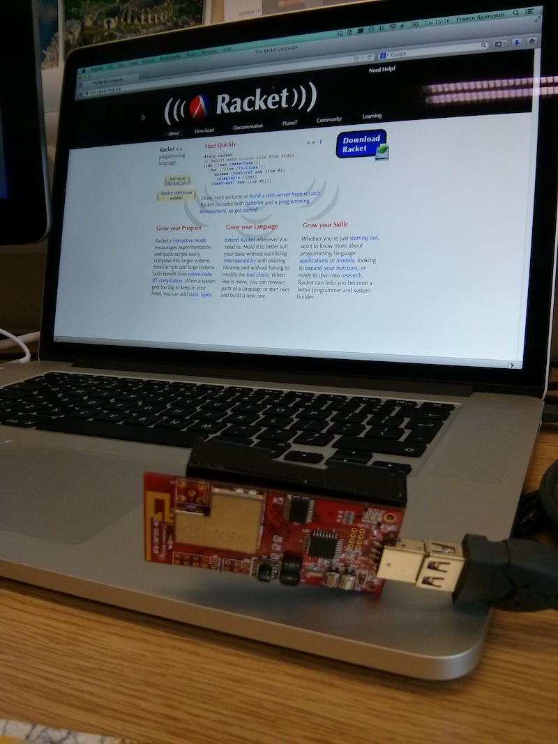
As an example, I start from a simple application that broadcasts temperature and humidity. The application can be installed on various motes (just 2 in my configuration) and then a base station collects all the readings. In my case the base station is connected to the PC using a USB port. In my configuration I have a Ubuntu virtual machine running on a Mac where I have configured the TinyOS environment and Racket is running in this virtual machine. The same code runs directly on Mac. We are only interested in the structure of the message being broadcasted. This is a small variation of the standard examples that can normally be found in a .h header file; in my example the header file contains the following:

1
2
3
4
5
typedef nx_struct BlinkToRadioMsg {
  nx_uint16_t nodeid;
  nx_uint16_t humidity;
  nx_uint16_t temperature;
} BlinkToRadioMsg;

This says that each message contains 2 bytes (16 bits) for nodeid, 2 bytes for humidity and 2 bytes for the temperature, for a total of 6 bytes. Messages are transmitted in TinyOS packets over the wire, and these packets have a special format. See Section 3.6 of the document available at http://www.tinyos.net/tinyos-2.x/doc/html/tep113.html if you want more information. In summary, a packet looks like this:

7e 45 00 ff ff 00 01 06 22 06 00 01 04 5c 18 69 37 6b 7e

where the sequence 7e is a reserved sequence to denote the start and the end of a packet. The actual payload (i.e., the 6 bytes we want to receive) in our case is the sequence “00 01 04 5c 18 69″, where “00 01″ is nodeid, “04 5c” are the two bytes for humidity and “18 69″ are the two bytes for temperature. The rest of the packet includes a CRC check, protocol ID, etc. See link above if you are interested in the details.

To read these packets I modify a little bit the code that is used in firmata.rkt to communicate with an Arduino board using firmata. The idea is simple: I create an input file attached to the USB port and I keep reading bytes. When I recognise a packet, I parse it an print the values of ID, humidity and temperature on screen. Let’s start by creating the input file:


1
2
3
4
5
6
7
8
9
10
11
12
13
14
15
16
17
18
;; This is the input file to be defined below
(define in null)
 
;; This is used to open the connection and to launch the reading loop
;; You typically launch it with (open-port "/dev/ttyUSB0)"
;; (check the port name with the command-line instruction motelist)
(define (open-port port-name)
  (printf "Racket-TinyOS starting... please wait\n")
 
  ;; This is used to associate the port to the file
  (set! in (open-input-file port-name #:mode 'binary))
  (if (system (string-append "stty -F " port-name " 115200 cs8 cread clocal"))
    (begin
     (read-loop) ;; see below for the definition of this
    )
    (error "Could not connect to " port-name)
  )
)

The (read-loop) simply reads one byte at a time and calls itself:

1
2
3
4
(define (read-loop)
  (process-input (read-byte in))
  (read-loop)
)

The function (process-input) is where the packet is built:

1
2
3
4
5
6
7
8
9
10
11
12
13
14
15
16
17
18
19
20
21
22
23
24
25
26
27
28
29
30
;; This is where we store the packet
(define packet null)
 
;; These are used to define the end-of-packet and start-of-packet sequences
(define sop #x7e) ;; start of packet
(define eop #x7e) ;; end of packet
 
;; These are used to record the fact that an end-of-packet 
;; (or start-of-packet) have been received
(define eop-rec 0) ;; end-of-packet received
(define sop-rec 0) ;; start-of-packet received
 
(define (process-input data)
  ;; First of all we add the byte to the packet
  (set! packet (cons data packet))
  (cond ( (and (= eop-rec 0) (= data eop))
          ;; If it is an end-of-packet sequence, we record it
          (set! eop-rec 1)
          )
        ( (and (= eop-rec 1) (= data sop))
          ;; If we find a start of packet after an end-of-packet we parse
          ;; the packet (we have to reverse it, because it was built in
          ;; the opposite order)
          (parse-packet (reverse packet))
          ;; and then we start again and we empty the packet.
          (set! eop-rec 0)
          (set! packet null)
          )
        )
)

Up to this point the code is re-usable for any packet content. In the function (parse-packet), instead, we have to process the bytes according to the message format defined in the header file (see above). This function is defined as follows:

1
2
3
4
5
6
7
8
9
10
11
12
13
14
15
16
17
18
19
20
21
22
(define (parse-packet packet) 
 
  ;; Very easy: ID is at position 10 and 11
  ;;            Humidity position 12 and 13
  ;;            Temperature position 14 and 15
 
  ;; These functions get the two bytes into the actual ID,
  ;; humidity and temperature. 
  ;; for the actual formula
  (define id (+ (* (list-ref packet 10) 256) (list-ref packet 11)))
  (define rh (+ (* (list-ref packet 12) 256) (list-ref packet 13)))
  (define temp (+ (* (list-ref packet 14) 256) (list-ref packet 15)))  
 
  ;; We then convert RH and temp according to datasheet for sensirion sht11
  (set! rh (+ (* rh 0.0367) -2.0468 (- (* 0.00000159 rh rh))))
  (set! temp (+ (* temp 0.01) -39.7))
 
  ;; Omissis: print the actual date. See link below for full code.
 
  (printf "~a ~a ~a\n" id rh temp)
  (flush-output)
  )

The final result of this code is the following output

2013/10/29 17:04:55 1 61.36022401 10.379999999999995
2013/10/29 17:05:02 2 35.30190249 23.799999999999997

Where the first number after the time is the node id, followed by the relative humidity, followed by the temperature. I have redirected this output to a file called office-all.txt for one hour, placing one sensor inside my office (with sensor id 2) and one sensor outside the office (sensor id 1). At the end of the hour I split this file with the command-line instruction

grep " 1 " office-all.txt > office-out.txt
grep " 2 " office-all.txt > office-out.txt

Then, I plot the temperature with the following gnuplot script:

set timefmt "%Y/%m/%d %H:%M:%S"
set xdata time
set terminal png font "/Library/Fonts/Arial.ttf" 28 size 1600,1200
set output 'office-temp.png'
plot "office-out.txt" using 1:5 title "Outdoor", "office-in.txt" using 1:5 title "Indoor"

This is the final result:

office-temp
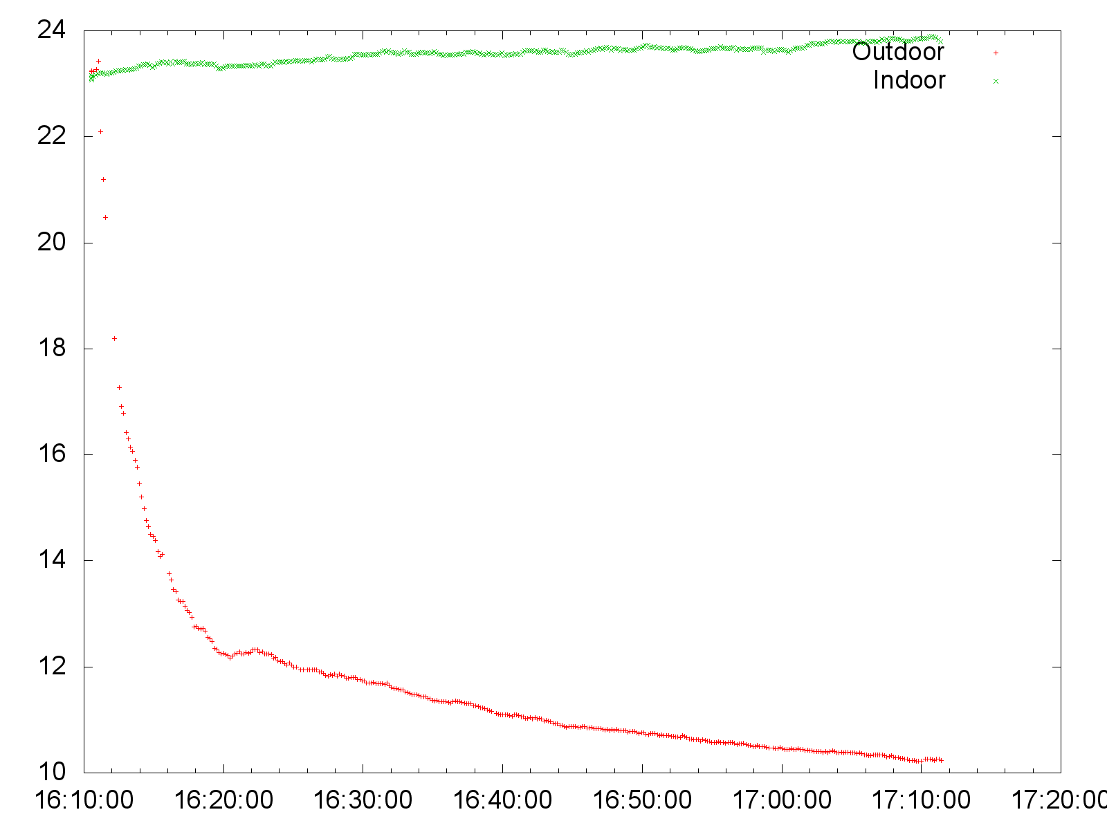
Notice how the indoor temperature remains constant (in green), while the outdoor temperature drops in 10 minutes when the sensor adjusts to the outdoor temperature, and it keeps decreasing as the sun sets. A very similar script for relative humidity produces this graph:

office-rh

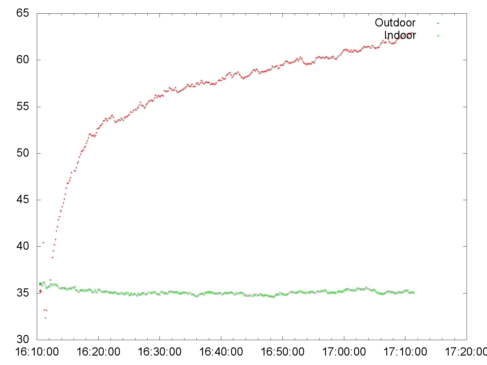
(notice how the relative humidity outside increases as the temperature decreases).

You can download the full Racket code by clicking here.

*** NOTICE!!! *** The parse-packet function is broken: it should take into account the escape sequences before parsing! I leave this to you to fix :-).

A very simple introduction to Fluxus and Fluxa

Screen Shot 2013-10-23 at 13.02.45This is a very simple write-up of my experiments with Fluxus and Fluxa to generate sounds (I don’t call it music…). It is intended for students who know a bit of Racket but have no experience at all with Fluxus and Fluxa. The results are just an example of what can be done, I hope someone will start from these to produce something better.

Back to Fluxus and Fluxa: if you have managed to install it (see my other post on How to Install Fluxus on Mac), make sure that you have Jack running and that you launch fluxa from the command line. Then, launch Fluxus and you can start with the experiments.
First, you need the following line:

(require fluxus-018/fluxa)

Then, you can start playing sounds immediately. For instance, try this:

(play-now (mul (sine 440) (adsr 1 1 1 1)))

The instruction above does the following: it generates a sinusoidal wave of frequency 440 Hz with the instruction (sine 440), and then it multiplies this signal with an adsr envelope with attack, drop, sustain and release all set to 1. If you are like me and don’t have an idea of what an adsr envelope is, please have a look at this simple introduction to synthesizers: http://beausievers.com/synth/synthbasics/

There are different wave forms available in Fluxa: in addition to sine, there is squ (square), tri (triangle) and saw. There are also white and pink noise generators.
It doesn’t stop here: you can use a lot of filters, including various moog filters. Have a look at this page if you are interested: http://www.pawfal.org/fluxus/docs/0.17/en/fluxa.html.

All these ingredients are typically put together in a loop to play music. In fluxa, you use the following construct:

(seq
  (lambda (time clock)
    (when (zmod clock 2)
      (play time (mul (sine (mul 100 (pow (adsr 0 0.1 0.8 1) 6)))
       (adsr 0 0.5 0.4 5))))
  0.5)
)

This is a loop that is repeated every 0.5 second. The lambda function has two parameters: the absolute time (in seconds, since the start of Fluxus) and an integer counter called clock.
The function (zmod clock 2) is true when the value of the clock is a multiple of two, i.e., every other iteration. As each iteration lasts 0.5 seconds, the play instruction is repeated every second; notice that here we use play and not play-now. Play takes and additional time parameter to specify when it should be executed. The magic combination of mutlipliers and adsr envelopes above generates a heart beat (I have copied this from one of the example available in the source code).

You can use fluxa to learn everything you need to know (and a bit more) about modulo functions, synchronization, and reasoning about time. These are some of the examples I have created:

  • Close Encounters of the Third Kind (CETK): just five notes repeated with increasing BPM. You can download cetk.scm here.
  • The SOB beat: instead of using the seq mechanism of fluxa, I use every-frame and plot a graph together with a beat for each SOB, more or less (a SOB is a “Student Observable Behaviour”, a new mechanism of assessment that we use for our undergraduate students of Computer Science; each student is supposed to demonstrate a certain number of SOBs during the year, and we record these using a dedicated tool from which I have exported the observations so far). The graph is equivalent to the one visible from our SOB admin dashboard, with students on the x axis and number of observed SOBs on the y axis. For each student I play a number of beats equal to the number of SOBs. This result in an increasing heartbeat. You can download SOB-beat.scm here and you can also watch a screen capture on Youtube at http://www.youtube.com/watch?v=WWMEfdbk4Kw (you may need to increase your volume)
  • The SOB melody: this is very similar to the previous one, but instead of playing a beat I play a note from a scale. For each student I change the scale in a random way (only 2 scales for the moment). You can download SOB-melody.scm here and you can watch the corresponding screen capture (with some live comments) here: http://youtu.be/1dO1CSgfpBc
  • Finally, back to the seq mechanism and a few operations with modulo: I take the list of SOB id in the order in which they are observed and I play them back in a random scale (selected at the beginning). You can download The delicate sound of sobs here.

Feel free to play around with these files and let me know if you obtain something better!

Installing Fluxus on Mac OS X 10.6-10.8

kleineFluxus is a “a live coding environment for 3D graphics, music and game” available at http://www.pawfal.org/fluxus/. If you know Racket (or LISP, or Scheme) it will look immediately familiar. I wanted to install it for our new Computer Science degree, where we teach Racket, and I wanted to do some experiments with its music capabilties. However, the installation is not exactly user-friendly… I have tried the precompiled package available from the website but sound did not work for me (flexa was missing). In the end, I installed the source files and compiled them, and I managed to have the sound.

This is what I have done on a Mac OS X 10.6 (a 6 year-old Mac Pro) and Mac OS X 10.8 (a 3-week old Mac Book Pro). It is essentially what the README file in the source tree tells you to do; the problem is that you find a lot of websites giving you different suggestions, including the README file itself. For instance, the README file tells you that you can use Homebrew to install fluxus, but the homebrew installation is broken for the moment… So, here it goes:

  • Install the 32 bit version of Racket, dowloadable from http://racket-lang.org/download/. I have installed 5.3.6. Notice that you really need the 32 version: fluxus will not link against the 64-bit version.
  • Install Macports from https://www.macports.org/install.php. This is needed to install all the fluxus dependencies below.
  • Clone the fluxus source code: git clone git://git.savannah.nongnu.org/fluxus.git
  • Add the following two lines to your .bash_profile:
    PATH=$PATH:/opt/local/bin:/Applications/Racket\ v5.3.6/bin/
    export DYLD_FRAMEWORK_PATH=/Applications/Racket\ v5.3.6/lib/

    Make sure that the Racket version is correct, and change it appropriately if needed.The file .bash_profile shoud be in your home directory, typically something like /Users/franco/. If it does not exist, just create it and make sure to open a new terminal so that these variables are loaded. You can check this with the command echo $PATH from the command line.

  • Install all the dependencies using macport. From the command line, run:
    sudo port install fftw-3 +universal glew +universal freetype \
      +universal jpeg +universal liblo +universal libpng +universal \
      libsndfile +universal ode +universal tiff +universal zlib \ 
      +universal scons

    (all this should be on a single line. If not, remember to add the backslash at the end). This will take a bit of time, don’t worry and have a coffee or tea in the meanwhile.

  • Install JackOSX from http://www.jackosx.com/. I have installed version 0.90 beta 15. This requires to reboot your computer, do this now and have another coffee or tea in the meanwhile.
  • Go back to the directory where you have downloaded fluxus. In this directory, type:
    scons ADDONS=0

    to compile fluxus. Again, you will need to wait a bit (but not too much, not enough for another coffee or tea). Scons is yet another building system that was installed using macports a few lines above.

  • Finally, you can install fluxus with:
    sudo scons ADDONS=0 install

You are now ready to test the sytem. You need to start Jack and fluxa, and then you’ll be able to play some music. More in detail:

  • In Applications, look for the folder called Jack, open it and double click on JackPilot. Check that the configuration is correct, save it, and then start JackPilot. Wait a few seconds and it should be ready, giving you CPU load.
  • In a terminal, launch the command fluxa (it should be in your path). It should just say “fluxa server ready”
  • Finally, let’s try to play something. In a terminal, go to the source tree of Fluxus, enter the “examples” directory, and at the command line type fluxus sound.scm. Press ctrl+e (or F5) and enjoy…

New academic year: welcome!

parliamenthill2

It is Sunday evening, and for a lot of students tomorrow will be the first day at Middlesex University. Formal lectures will only start on the 7th of October, but from tomorrow “induction week” is on and students will get their access cards and will go through a lot of activities, meeting staff members and other students.

This year I teach “Information Security Management” for MSc students in Electronic Security and Digital Forensics. I will talk about this in another post at some point in the future.

More importantly, tomorrow will be the first day for our new undergraduate Computer Science programme. This is a completely new programme: in their first year, students will use Racket, Arduino boards, Rasperry Pi, and a will do a lot of interesting things, including reading and posting tweets from a robot…

I still remember my first academic year and I can also remember my very first days at university. Given that the first days are so important (see the Baby duck syndrome for an interesting article on imprinting and software), we have decided to make this first week a bit different… We will work with students to learn the basic ingredients of LaTeX, “the de facto standard for the communication and publication of scientific documents”. LaTeX is a simple example of a programming language, and this is a simple example of LaTeX program:

1
2
3
4
5
6
7
8
9
10
11
12
13
14
15
16
17
18
19
20
21
22
23
24
25
\documentclass{article}
 
\begin{document}
 
\title{Hello World!}
\author{Franco Raimondi}
 
\maketitle
 
\section{Introduction}
Printing Hello World is usually the first thing you learn in a programming language.
 
\section{Another section}
 
You probably know this equation:
\begin{equation}
E=mc^2
\end{equation}
 
This is another very important equation:
\begin{equation}
i \hbar \frac{\partial}{\partial t} \Psi = \hat{H} \Psi
\end{equation}
 
\end{document}

With LaTeX you do not worry about the actual output, but you simply say that “Hello World” (line 5) is a title, that the Author is Franco Raimondi (line 6), that there is a section whose title is Introduction (line 10), and that the content of the section is “Printing Hello World is usually the first thing you learn in a programming language.” (see http://en.wikipedia.org/wiki/Hello_world_program if you want to know more). At line 13 another section begins, containing two equations (the syntax of equations in LaTeX will not be covered, but you can find plenty of documentation on-line).

In the labs, students will compile LaTeX code and generate PDF files using one of the many compilers available such as MiKTeX and TeXnicCenter, learning that the compiler takes care of the actual result.

Click on this link to see the final result for the example above.

Finally, if you have Facebook or Twitter, don’t forget to follow these two pages:

Book Review: The Golden Ticket

The Golden Ticket: P, NP, and the search for the impossible
by Lance Fortnow

I had this book on my bedside table for the past two months. As you can see, I did not have time to write anything here since the end of April: the end of term, exam marking, exam boards, a long list of project deadlines and reviews for various conferences meant that I had to postpone almost everything that was not urgent, including the removal of items from the stack on my bedside tabale (the actual structure of the pile of items is an interesting topic of research on its own: see exercise below).

An eleven hours flight to San Francisco is the perfect environment to read this short book, to write this post, and to make my wife slightly less upset about the status of my bedside table: hopefully I’ll be able to empty it by the end of summer so that dust can be appropriately removed without the need of finding the shortest path among all the obstacles I leave on it.

Back to the book: it starts with the observation that “there seems to be no limits to what computers can do. Or is there? [The] book explores the computational problems that we may never be able to compute easily“.

The bold is mine, because this is the key issue: some problems have solutions that are “easy” to compute, some others are difficult.  The book is not about undecidable problems (see my other post www.rmnd.net/the-universal-computer/ for a reference), but about the complexity of problems for which a solution exists. The book avoids all the technical details of complexity classes expressed in terms of Turing machines and focuses instead on two of them: the class of “easy” problems called P (because they can be solved with an algorithm that runs in time polynomial in the size of the input), and the class of problems for which a solution cannot be computed easily but, when a solution is given, its correctness can be verified easily. This latter class is called Non-deterministic Polynomial, because when a solution can be guessed, it can be verified in polynomial time. If you are interested in the mathematical details, I recommend the book “Computational Complexity” by Christos Papadimitriou.

One of the fundamental questions in Computer Science and in Mathematics is: are the two classes P and NP equal or different? This is the question that the book explores with captivating examples and a presentation that is suitable for everyone.

Chapter 3 provides examples of problems in P (matching problems, shortest and Eulerian paths, min-cut) and so-called NP-complete problems (Hamiltonian cycles, four colour problem, max-cut). I know my list may sound boring, but the presentation in the book is full of clear and funny examples. Additional hard problems are described in Chapter 4, including games such as Minesweeper, Tetris and Sudoku, the satisfiability problem and the works of Cook, Karp and Knuth.

Chapter 6 presents in a very clear way some of the techniques that can be used to solve “difficult” problems in NP, and Chapter 7 describes some of the techniques that have been employed to tackle the P vs. NP problem. This latter chapter, together with Chapter 5, are my favourite in the book: they provide the historical context in which the problem was born, and they give an account of both the Western and the Eastern research groups involved. This is something you don’t find in standard textbook and is one of the reasons you should read this book even if you already familiar with computational complexity (in addition to a very useful list of examples that can be used for teaching purposes)

Chapters 8 to 10 take a detour in cryptography and quantum computing, presenting the important connections between these topics and complexity theory, and concluding with a list of challenges for the future that go beyond the P=NP question.

Franco, did you buy a faulty book without chapter 2? Why are you not talking about it?
Because I think it should have been more formal. The chapter talks about an ideal world in which P is equal to NP: in this world it would be possible to cure cancer and to forecast weather at any time in the future. I don’t think this is the case. I am not an expert in DNA sequencing, but I know something about weather forecast: in this case reliability is not related to the complexity of finding a solution, but to the problem of the dependance from initial conditions (the famous butterfly effect). Even if we had a polynomial algorithm for weather forecast, I think this would not solve the issue of the uncertainty of result given the sensitivity on initial conditions.

So should I read the book or not?
You should definitely read it! The book is excellent, a pleasure to read and full of very interesting and useful information. I personally did not like the style of chapter 2, but this is the only issue I had (and it could be that other people like that chapter); I really enjoyed everything else.

The Golden Ticket
P, NP, and the search for the impossible
by Lance Fortnow
Princeton University Press, 2013

Continue reading

Mushrooms and the universal vs. existential “eventually”.

Today I gave the last lecture of my course “Logic and Model Checking”. In the past few weeks we have revised Computational Tree Logic (CTL) and I spent a bit of time explaining the difference between the semantics of the CTL operators AF and EF. The first one expresses the universal “eventually”: if you write AF p, this means that “for All paths”, “at some point in the Future”, the proposition p will be true. EF p, instead, means that “there Exists a path” such that “at some point in the Future”, the proposition p will be true.

The standard example I use the explain the difference is to set p equal to the proposition “find a mushroom”. So, “AF p” means: it doesn’t matter which path you take, just be patient and you will eventually find a mushroom. “EF p”, instead, means: there exists a path such that, if you follow that path, you will eventually find a mushroom. I then go on explaining that my only way of finding an edible mushroom is to be in a wood where AF p is true, because in “EF p” woods I will never find a mushroom (I am really unlucky at mushroom hunting).

I guess the students liked the analogy, this is what I got today at the end of the class:

2013-04-23 16.32.33

It is now my turn to revise an old recipe I used to prepare: Portobello mushrooms with goat cheese.

Repast Simphony (Java): a quick overview + installation instructions

I started playing with Repast Simphony both for research and for teaching. This is a first post that includes  a quick overview (part I) and some installation instructions (part II). Hopefully I will be able to add more details  in the future.

Part I: Quick overview

Repast Simphony 2.0 is an “agent-based modeling and simulation platform”. Using this platform agents can be modelled using ReLogo (a dialect of Logo), flowcharts, Groovy, or Java.  Notice that there is also a Repast for High Performance Computing “intended for large-scale distributed computing platforms” using C++. Here I am only looking at Repast Simphony, and only at Java as a modelling language.

The tutorial available at http://repast.sourceforge.net/docs/RepastJavaGettingStarted.pdf provides a step-by-step guide for building a simple application called jzombie. I’m not going to go through this tutorial in detail. Instead, I highlight some of the key features of this framework using the example from the tutorial.

In Repast agents are created as simple Java classes with the use of some Repast-specific methods. For instance, this is an excerpt of the Human class in jzombie:

1
2
3
4
5
6
7
8
9
10
11
12
public class Human {
  private Grid<Object> grid;
  // [...]	
 
  @Watch(watcheeClassName = "francojrepast.Zombie",
	watcheeFieldNames = "moved",
	query = "within_moore 1",
	whenToTrigger = WatcherTriggerSchedule.IMMEDIATE)
  public void run() {
          // [...]
  }
}

Human agents live in a Grid (a Repast Class), and the simulator invokes the method run() whenever the condition specified in the @Watch annotation becomes true (intuitively: whenever a Zombie is at distance 1). Zombie agents are modelled in a very similar way and they implement a method step() that is invoked at every step in the simulation (see the tutorial for the full code). All the agents are defined in a context, as exemplified by the following code:

1
2
3
4
5
6
7
8
9
10
11
12
13
14
15
16
17
18
19
20
public class JZombiesBuilder implements ContextBuilder<Object> {
 
  @Override
  public Context build(Context<Object> context) {
  // [...]
    int xSize = (Integer)params.getValue("x_size");
    int ySize = (Integer)params.getValue("y_size");
    int zombieCount = (Integer)params.getValue("zombie_count");
    int humanCount = (Integer)params.getValue("human_count");
    // [...]
    for (int i = 0; i < zombieCount; i++) {
      context.add(new Zombie(space, grid));
    }
    for (int i = 0; i < humanCount; i++) {
      int energy = RandomHelper.nextIntFromTo(400, 1000);
      context.add(new Human(space, grid, energy));
    }
    // [...]
  }
}

The method build() reads parameters from the simulator (see below) and creates the appropriate number of agents (notice the use of the Repast class RandomHelper to generate random values for energy levels of humans). Agents are added to the context that, in turn, is created by the simulator. The Repast simulator is invoked from Eclipse (see tutorial for the details), and this is what it looks like after it starts:

Screen shot 2013-04-17 at 17.03.29Notice that these are the same parameters specified in the context Builder above. The simulator can be configured to display the grid and, by running it, it is possible to follow the evolution of the system. This what the grid looks like at the beginning of the simulation:

Screen shot 2013-04-16 at 17.20.43

It is possible to add a number of features to the simulator. For instance, it is possible to create data collections (such as counting the number of agents) and to display time series. This is an example of the total number of Humans and total number of Zombies over time:

Screen shot 2013-04-16 at 17.21.33

It is also possible to define connectors with external tools, such as R, Excel, and generate SQL code. This is what I am planning to do next.

Part II: Installation Instructions

First of all you need to download the tool, which essentially runs as an Eclipse plug-in. Depending on your platform, this is what you need to do:

  • Mac OS X: just download the 64-bit image or the 32-bit image and follow the very easy instructions. This will download a (large) image containing Eclipse 3.7 and all the necessary plug-ins already installed.
  • Windows: download and run the Windows Installer (I have not tried this, but I assume that it is similar to Mac OS X)
  • Linux: this is slightly more complicated:
    • You need to download Eclipse. I used a fresh copy of Eclipse 3.7 Classic 64 bit (a 32 bit version is also available).
    • You then need to install Eclipse XML Editors and Tools: click on Help -> Install New Software, then click in “Work with” and select “All Available Sites”. Scroll down the list, expand “Programming Languages” and select “XML Editors and Tools”. Complete the installation and restart Eclipse as required.
    • You then need to install Groovy using a local archive. Download this zip archive and expand it somewhere on your disk. Go back to “Help -> Install New Software”, now click Add, select Local, and browse to the directory you have just created. Select all items and install them. Again, Eclipse will restart.
    • At this point you can install Repast Simphony. Once more, click on “Help -> Install New Software”, select Add and in Location copy this link: http://mirror.anl.gov/pub/repastsimphony. Select everything, install and restart Eclipse.

If everything went well, you can now start the platform. If you are using Mac, you will find Repast in your Applications folder. If you are running Linux, just start Eclipse. You can create a new Java Repast project with File -> New -> Other, open Repast Simphony and choose “Repast Simphony Project”. At this point you can go back to the tutorial.


Who is talking about pizza in London?

Some of my students are interested in using Twitter data for their projects, and some others are interested in developing network applications. In this post I show how to retrieve data from the Twitter stream and how to manipulate it with server-side Javascript using node.js. In particular: I will build a stream of all the geo-tagged tweets from London talking about pizza.

DISCLAIMER: I am not an advocate of node.js. The same thing could be done in Python, Ruby, you-name-it. I am using node.js because 1) my students are familiar with Java and 2) the code is very short.

OK let’s start from a quick introduction to the Twitter stream API: there is a sample stream available from https://stream.twitter.com/1/statuses/sample.json. This stream will return a random sample of tweets (notice: this is a lot of data!). You can connect to this stream in a number of ways, the easiest is from the command line using curl (this works on Mac and Linux, I don’t know in Windows. You obiously need to have a Twitter account for this):

$ curl --user YOURUSERNAME:YOURPASSWORD https://stream.twitter.com/1.1/statuses/sample.json

This will display a long list of tweets in JSON format. You can even point your browser to this address and see what happens. From the command line you could redirect the output to a file to be processed at a later stage, but it is probably a better idea to retrieve only the tweets that are relevant to you.

In my case, I am interested in tweets originating from London and containing certain keywords. Twitter provides an end-point for this, see https://dev.twitter.com/docs/api/1.1/post/statuses/filter. In particular, one can retrieve all the tweets containing specific keywords, or originating from a certain location (assuming the user provides this information). Again, there are a number of ways to connect to this end-point. If you want to use Python, there is a very simple class called tweetstream that can help you with this; otherwise, you can still use curl passing the parameters in the appropriate way:

curl --user YOURUSERNAME:YOURPASSWORD -d "track=pizza" https://stream.twitter.com/1.1/statuses/filter.json

Irrespective of the technology you use to connect, there are two key things to keep in mind:

  1. The filtered stream is not a sample, it’s the full set of tweets satisfying your query (subject to certain limits).
  2. If you provide more than one condition (e.g. a location and a list of keywords), the API will return all the tweets satisying any of the two. If you want the tweets that satisfy both conditions (e.g., all the tweets talking about pizza in London) you need to retrieve all the tweets from London, and then filter them locally. This is what I am going to do below.

Let’s now move to retrieving the tweets and displaying them in real time. Download node.js for your platform from this link: http://nodejs.org/download/ (I am using the binary version 0.10.1)

Extract the archive and try to write a simple http server. This is taken from http://nodejs.org/ and is a simple http reserve running on port 8080 and returning the string Hello World! to all requests:

1
2
3
4
5
6
var http = require('http');
http.createServer(function (req, res) {
  res.writeHead(200, {'Content-Type': 'text/plain'});
  res.end('Hello World\n');
}).listen(8080, 'YOUR IP ADDRESS HERE');
console.log('Server running at http://YOUR IP ADDRESS HERE:8080/');

(obviously: put your IP address in the right place and make sure you don’t have firewalls blocking port 8080 etc). Save this code in a file, for instance test.js, and then run it with:

$ /path/to/node/bin/node test.js

Point your browser to the IP address on port 8080 and you should see Hello World!

The next step is to connect to the Twitter streaming API using node.js. To this end, I use this client: https://github.com/ttezel/twit. Just get it and install it (follow the on-line instructions, it should be very easy).

Before connecting to the Twitter API, go to https://dev.twitter.com/apps/new and create an application. You need to get a consumer_key, a consumer_secret, an access_token, and an access_token_secret. At this point you can connect to the Twitter streaming filter with the following code:

1
2
3
4
5
6
7
8
9
10
11
12
var Twit = require('twit')
var T = new Twit({
    consumer_key:         '...'
  , consumer_secret:      '...'
  , access_token:         '...'
  , access_token_secret:  '...'
})
var london =  [ '-0.489','51.28','0.236','51.686']
var stream = T.stream('statuses/filter', { locations: london })
stream.on('tweet', function (tweet) {
  console.log(tweet)
})

Fill in your keys, save the file and try to run it: you should see a stream of tweets from London (the bounding box is derived from openstreetmap).

I now put the two things together: I will stream the tweets using an http server. The code is the following:

1
2
3
4
5
6
7
8
9
10
11
12
13
14
15
16
17
18
19
20
21
22
23
24
25
26
var Twit = require('twit')
var http = require('http')
var url = require("url")
 
var T = new Twit({
    consumer_key:         '...'
  , consumer_secret:      '...'
  , access_token:         '...'
  , access_token_secret:  '...'
})
 
var london = [ '-0.489','51.28','0.236','51.686']
var stream = T.stream('statuses/filter', { locations: london })
 
var server = http.createServer(function (req, res) {
  var uri = url.parse(req.url).pathname;
  if(uri === "/pizzastream") {
    console.log("Request received");
    stream.on('tweet', function(tweet) {
      if(tweet.text.toLowerCase().indexOf("pizza") &gt; -1) {
        res.write(tweet.user.name+" says: "+tweet.text);
      }
    });
  }
});
server.listen(8080);

The code is as follows: line 13 creates a variable called stream that includes the stream originating from the Twitter API. Line 15 creates a variable called http for the http server. In line 16 and 17 we check whether the requested URL is /pizzastream. If this is the case, every time there is new data on the Twitter stream (line 19), if the text of the tweet contains the word “pizza” (line 20), I write the name of the user and the text of the tweet to the http stream (line 21). Notice how the value of the various fields is accessed using tweet.text and tweet.user.name (other fields are available, check the full JSON output). You can check the actual output by pointing your browser to the address of the machine running this code, for instance http://192.168.0.10:8080/pizzastream.

The code should be improved to include an “else” statement for the if condition in line 17. Also, the stream should be kept “alive” when there is no data: have a look at the documentation available at this link: http://nodejs.org/api/stream.html

The nomadic board

(a long post on my panoply of teaching tools.)

When I started teaching in the UK more than 10 years ago, I was a teaching assistant at King’s College for Foundations of Computing and for a number of other courses. I was using chalk on a blackboard (to be precise: a green board), and in some rooms I was using an OHP with slides and a marker. Students didn’t have laptops and phones didn’t have internet.

A number of things have changed: here are Middlesex there are no blackboards, there are a few OHP left (a lot of times without slides), students have smartphones and in some cases I have to teach in rooms without (white) boards. The only certainty I have is that in every room there is a projector, a networked PC and video input for a laptop; the other certainty is that students are very likely to be connected using a phone or a tablet or a laptop (quite often a combination of these).

For sure, it is not possible for me to use the same teaching tools I used at King’s. There are two things that I can do:

  • start moaning
  • adapt

I am not going to express an opinion on which situation is better but, after a while, moaning is boring even for the moaner: I decided to adapt.

My first consideration is that there is no way for me to ban smartphones and other internet-connected gadgets from the room. Therefore, I decided that it could be a good idea to employ them, and this is what Lalith and I did a few months ago: http://q.mdx.ac.uk/about.php

The mechanism is simple: I can prepare questions in advance and advertise them to students at the right point in the lecture. Students then need to use their devices to answer the questions. This is an example of what students see on their devices (this is optimized for small devices):

Click here to answer: http://q.mdx.ac.uk/ox51g


And this is what I see as students answer, live in the class:

Results for a question about high order functions in Haskell

(It was quite clear that only half of the class could get the type right, so I spent a bit more time on high order functions during the labs).

The short code that I advertise to students is OK (5 characters in total), but it is probably too long to get it right most of the time. So, my second consideration was: let’s use Twitter to advertise the questions and other messages to students; a number of courses around the world are already doing this, so it is probably not a bad idea… Notice the small Twitter (and Facebook, if you prefer) buttons above in our application: these allow to share the question with a simple click (by me). I have created a Twitter account for my modules (https://twitter.com/cmt4031 and https://twitter.com/bis4610), and this is where I post the questions. In this way, students only have to follow the course, and they will receive the links directly: no need to type, they just need to open their Twitter stream during the lectures.

There was another problem left: the lack of a board. This would be a big change for me, I definitely need a board to make examples, respond to questions and do exercises. As usual, I had an idea while running: use a tablet. I have a Samsung Galaxy Note 10.1: I have this one because I wanted something where I could write using a pen (note: the iPad and other tablets will not work, you really need a tablet with a dedicated pen to have the adequate resolution). I used the tablet to annotate reports and theses, can it be used as a board? YES it can! And it works great: you only need to mirror the tablet on a desktop (or on a laptop) connected to the projector, and you have a board (see “Technical details” below for additional information).


The nomadic syntax of First Order Logic (lecture in room C215, no board, using my Linux laptop with vinagre). The big screen is out of focus, but I guarantee it is readable.

In this way you have more than a board: you have what I decided to call a “nomadic board”. You can walk around the room, sit with the students, move around, sit somewhere else, etc. My current workflow is the following: I do not project the slides, even if these are available online and students can see them if they want (possibly using their devices, possibly during the lecture). Instead, I write the key elements of the slides on the “board” (definitions, etc.), walking around and sitting with students while I do this. If there is a question, or if I ask a question using q.mdx.ac.uk, I explain the answer using the “board”. At the end of the lecture I upload all the notes from the “board” as a PDF file to our VLE so that students have these available (in addition to the standard slides).

There is an additional benefit. In Italy, it was quite common to be “called to the board” to solve exercises. The teacher / lecturer / teaching assistant would pick a random student and ask to solve an exercise. I used to do this, but I stopped a few years ago as it was impractical to switch between slides projected on a screen and the whiteboard. But now I can do this again, just a bit differently: instead of asking the student to walk to the board, I walk the “board” to the student:


Michael (CMT4031 student) hard at work to encode mutual exclusion on the tablet (H104 lab, using the Windows 7 desktop in the room with RealVNC)

Typically, I ask “what is the day today? 28th of January?”, and I look for the 28th student from left or right; I have a number of variations on this (“what is your day of birth”,  add the two digits, and so on), so that students cannot choose their seats according to the day.

Overall, this is working quite well and I’m happy with the current situation. Setting up the whole mechanism requires a bit of IT knowledge, so I’m not sure that the technology is ready to be adopted by everyone (see the “Technical details” below). But I guess that, eventually, the integration of tablets with projectors will become more common.

What if projectors are removed? Well, I’ll adapt once more…

Technical details.

Continue reading

Book review: The Universal Computer

I saw this title on a tweet by an Italian friend a couple of months ago, and I decided to add it to my queue of books-to-read, thanks to various positive reviews that are available online:

Martin Davis, The Universal Computer: The road from Leibniz to Turing.
Published by W. W. Norton & Co., 2000. 270 pages

I have now finished it and I can  say that this is not a good book: this is an extraordinary book about the history of computer science, and it should be compulsory reading in any CS curriculum.

The book provides an overview of a number of key figures in the history of mathematics and computer science: Leibniz, Boole, Frege, Cantor, Hilbert, Godel and Turing, with two final chapters on “hardware” history and directions for the future. What makes the book unique is that the presentation of the various philosophers and mathematicians is as captivating as the best novel you have ever read: it is just not possible to stop reading it. In fact, I am currently late with a couple of reviews that I planned to complete on a Eurostar trip because I had to finish this book.

The presentation is self-contained, no background knowledge is required to understand the various chapters (neither of philosophy nor of mathematics  / computer science). The description of the proofs of incompleteness for PA and undecidability for FOL are probably the most accessible I have ever seen (don’t forget to have a look at all the notes at the end of the book: they are as clear and as important as the main body of the book).

It is true that the book does not give an in-depth analysis of the various philosophers. It is true that some figures are missing (e.g., no mention of Tarski in “Beyond Leibniz’s Dream”). It is also true that the approach is a bit Manichean in some points (and in some cases my personal opinions are probably on the “wrong” side). Nevertheless, I think this book is fundamental to understand our position in history, what we do, and why we do it.

Overall, I think this book should be at the top of your reading list, right next to ZAMM.